

Introduction
This article is the second in a series and in our previous one, we performed Exploratory Data Analysis on time series data loaded using the Refinitiv Data library and PyCaret. In this article, we will make use of the AutoML functions available in PyCaret, to generate an evaluate an optimal predictive model or blended (ensemble) structure.
Refinitiv Data Library
The Refinitiv Data Library for Python provides a set of easy-to-use interfaces offering developers uniform access to the breadth and depth of financial data and services available on the Refinitiv Data Platform. The platform itself connects to the layer of data services providing streaming and non-streaming content, bulk content and even more, serving different client types from the simple desktop interface to the enterprise application. With the Refinitiv Data Library. The same Python code can be used to retrieve data regardless of which access point you choose to connect to the platform.
PyCaret
PyCaret is an open-source, low-code machine learning library in Python that automates machine learning workflows. It is an end-to-end machine learning and model management tool that speeds up the experiment cycle exponentially and can make you more productive. It is essentially a Python wrapper around several machine learning libraries and frameworks such as scikit-learn, XGBoost, LightGBM, CatBoost, spaCy, Optuna, Hyperopt, Ray and more, and it recently released a Time Series Module which comes with a lot of handy features that make time series modeling a breeze.
Pre-requisites
To run the example in this article we will need:
- Credentials for Refinitiv Data
- Anaconda
- Python 3.7.* as the PyCaret package used is compatible with this version
- Required Python Packages: refinitiv-data, pycaret-ts-alpha & pandas
Load Data
We already did the environment setup and installed required packages in our previous article. If you haven't done the setup, please refer to Environment Setup section in the previous article.
Import Packages
Lets import the packages we need for this example:
import warnings
warnings.filterwarnings('ignore')
import pandas as pd
from datetime import date, timedelta
from pycaret import time_series as ts
from pycaret.time_series import TSForecastingExperiment
import refinitiv.data as rd
from os.path import exists
rd.open_session()
df = rd.get_history(universe=["GOOG.O"], fields=['TR.PriceClose'], interval="1D", start="2014-01-01", end="2022-05-12")
rd.close_session()
df.reset_index(inplace=True)
df.head()
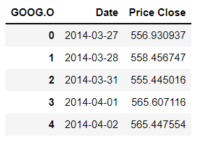
sdate = [int(i) for i in df.Date.min().split("-")] # start date
sdate = date(sdate[0], sdate[1], sdate[2])
edate = [int(i) for i in df.Date.max().split("-")] # end date
edate = date(edate[0], edate[1], edate[2])
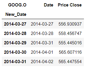
Next, lets set the new date column as the index and sort the data using it.
df['New_Date'] = pd.date_range(sdate,edate-timedelta(days=1),freq='d')[:df.shape[0]]
df.index = pd.PeriodIndex(df.New_Date, freq='D')
df = df.drop("New_Date", axis=1)
df['Price Close'] = df['Price Close'].astype(float)
df.sort_index(ascending=True, inplace=True)
In the above code, we converted the index type to PeriodIndex with Daily frequency and sorted the data by index which in our case here is the New_Date . Below is the snapshot of the final dataset:
df.head()
Modeling
In this section, we are going to pick the ARIMA model from above, and train it manually. But before that, let's explore a bit more about ARIMA models.
Autoregressive Integrated Moving Average
ARIMA (AutoRegressive Moving Average) belongs to a class of statistical models used for analyzing and forecasting time series data. Any ‘non-seasonal’ time series that exhibits patterns and is not a random white noise can be modeled with ARIMA models.

As we can see from the above equation, the target variable Yt is modelled as a constant plus the linear combination Lags of Y (up-to p lags) plus a linear combination of the lagged forecast errors (up-to q lags)
An ARIMA model is described using 3 hyperparameters (p, d, q):
- Autoregression: Uses the dependent relationship between an observation and some number of lagged observations. p is the order of the AR term
- Integrated: In order to make the time series stationary, subtracting an observation from an observation at the previous time step. q is the order of the MA term
- Moving Average: Uses the dependency between an observation and a residual error from a moving average to lagged observations. d is the order of differentiation required to make the time series stationary.
Pre-Defined Variables
Next let's define some global plot settings for figures and set some pre-defined variables, e.g., we are setting the value for forecast horizon to 30 days and number of folds for cross validation to test the models to 60.
fig_kwargs={'renderer': 'notebook'}
forecast_horizon = 60
fold = 3
Experiment Setup using Pycaret's TSForecastingExperiment
Now, let's initialise the setup using Pycaret's new object-oriented API. The Setup function initializes the training environment and creates a transformation pipeline. It takes two mandatory parameters: data and target, all the other parameters are optional.
exp = TSForecastingExperiment()
exp.setup(data=df['Price Close'], fh=forecast_horizon, fold=fold, fig_kwargs=fig_kwargs, session_id=123)
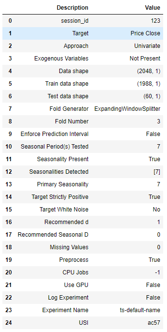
There is quite a bit of information shared during initialisation, more specifically:
We can see that our data has 2048 data points and pycaret kept the last 98 as a “test set” for out-of-sample forecasting. The remaining 1950 data points are used for training purposes.
Pycaret, after testing for seasonality, detected a primary seasonality of 7 days.
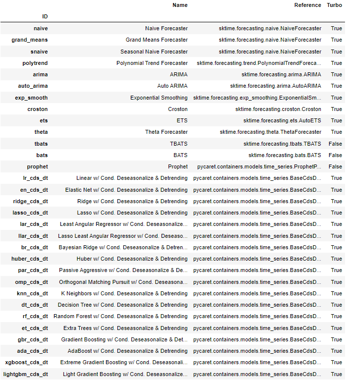
exp.models()
ARIMA models - An Introduction
In this section, we are going to pick an ARIMA model and train it manually.
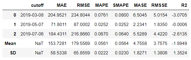
arima = exp.create_model('arima')
arima
Next, we are going to use auto tune capabilities to the above trained model to improve performance. If there is a possibility of improvement, the model will be tune its hyperparameters otherwise it will retain it's initial state.
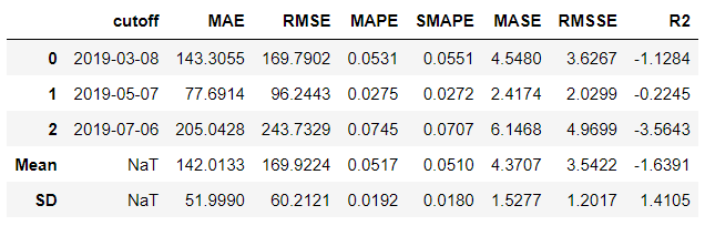
tuned_arima = exp.tune_model(arima)
tuned_arima
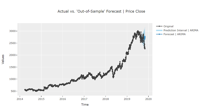
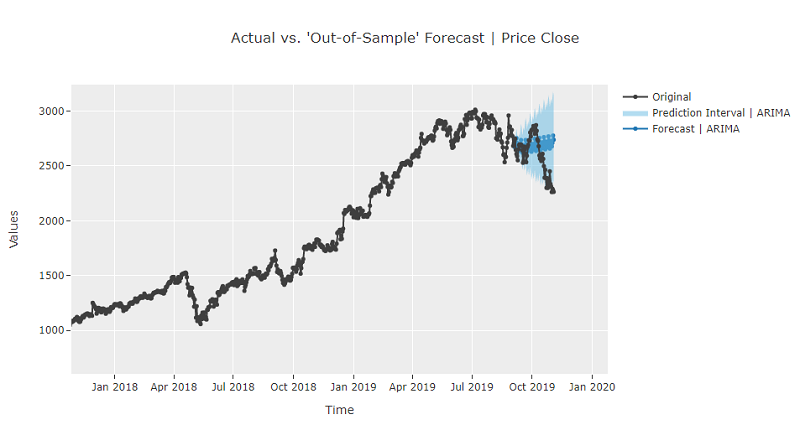
exp.plot_model(tuned_arima, plot = 'forecast')
AutoML
PyCaret provides as with many models to choose from and the Compare function trains and evaluates the performance of all the estimators available in the model library using cross-validation. The output of this function is a scoring grid with average cross-validated scores. By default, it returns the best model, however we can ask for the n top models to be returned using the n_select parameter.
best = exp.compare_models()
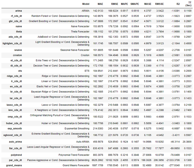
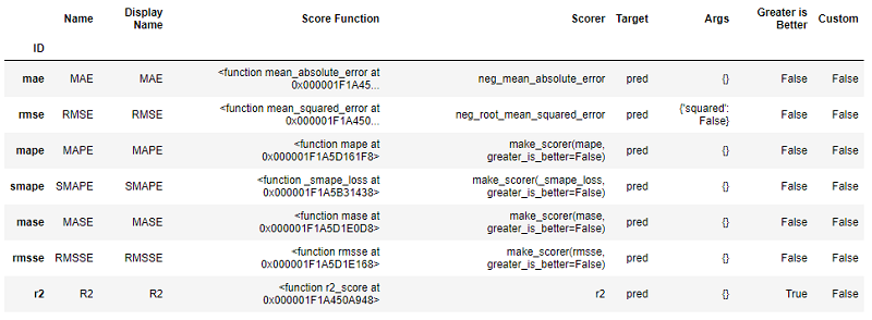
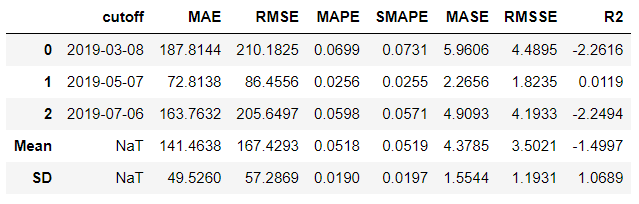
All the metrics used for evaluation during cross-validation can be accessed using the get_metrics function.
exp.get_metrics()
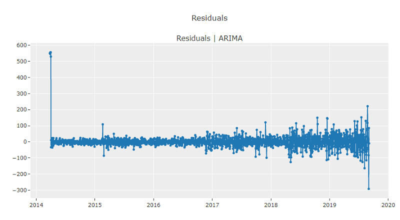
Let's generate a few plots on the best model. We can plot diagnostics by passing the model (estimator) to the plot_model., or ask for a residuals plot.
exp.plot_model(estimator=best)
exp.plot_model(estimator=best, plot = 'residuals')
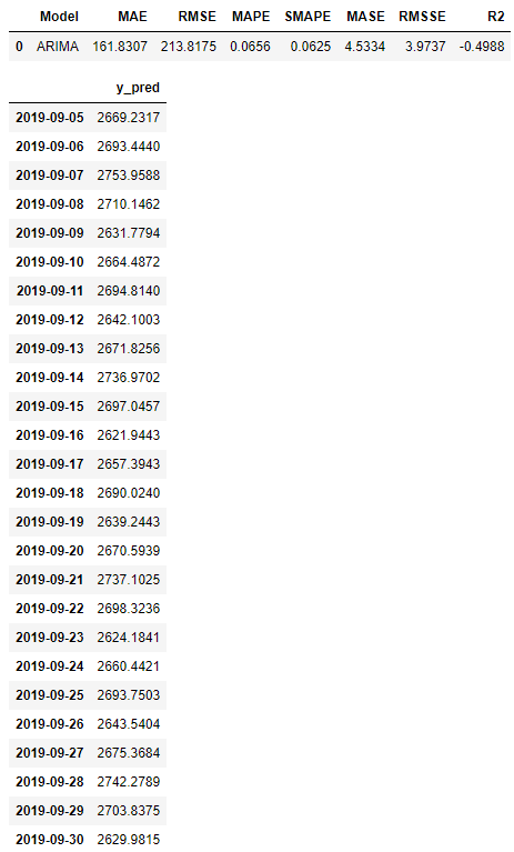
exp.predict_model(best)
best_baseline_models = exp.compare_models(fold=fold, sort='mae', n_select=3)
best_tuned_models = [exp.tune_model(model) for model in best_baseline_models]
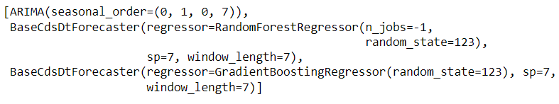
Blended Models
By using ensembles, the combination of several good models, we can achieve even better results. To do so in PyCaret we use the blend_model functionality. There are several options such as:
- Mean and Median blenders calculate the mean and median respectively of all individual model forecasts and uses that as the final forecast
- Voting blender will combine the individual forecasts using the respective weights provided by the user
top_model_metrics = compare_metrics.iloc[0:3]['MAE']
display(top_model_metrics)
top_model_weights = 1 - top_model_metrics/top_model_metrics.sum()
display(top_model_weights)
blender = exp.blend_models(best_tuned_models, method='voting', weights=top_model_weights.values.tolist())
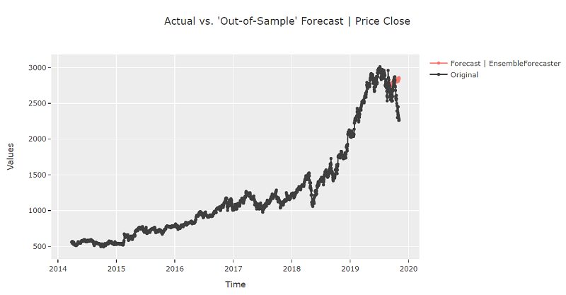
Let's now use the blended models for forecasting:
exp.plot_model(estimator=blender)
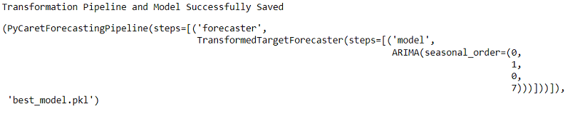
final_best = exp.finalize_model(best)
exp.save_model(final_best, 'best_model')
Finally, all we need to do to load and use the saved model, is write the following code snippet:
loaded_exp = TSForecastingExperiment()
loaded_model = loaded_exp.load_model("my_best_model")
loaded_exp.predict_model(loaded_model, fh = 30)
Conclusion
This Blueprint gives us a good foundation on how to use the RD library and PyCaret for AI modeling. After loading data using Refinitiv Data library, we engineered the missing data issues for non-trading days.
Furthermore, we trained multiple models using a single function call provided by time series module in PyCaret. We also fine-tuned the top 3 models for better results and even used a blended version of the models for better accuracy during prediction.
We saw how easy it was to use the automated approach to model the data and we were able to achieve reasonable results compared with the manual approach.
We also saved and loaded the model with a simple function call using PyCaret.
Please note, since this Blueprint is just for methodology understanding purposes, we haven't focused more on improving forecasting accuracy.