
Authors:

Overview
In this article, I extend on the Mergers and Acquisitions (M&A) predictive modeling that has been published earlier, by incorporating Natural Language Processing (NLP) based news sentiment variable into it. The original model used only financial variables and utilized Logistic regression for M&A target identification and showcased if that produces an abnormal return for investors. Instead, the purpose of this article is to test if news sentiment derived by NLP has any significant contribution to M&A predictive modeling. To do that, the significance (by comparing evaluation metrics) of news sentiment is tested on different Machine Learning (ML) models, including logistic regression, random forest, and XGBoost models. As it comes to the NLP model, Finbert and BERT-RNA models are tested to calculate sentiment on the news preceding M&A announcement.
The motivation behind using the news sentiment variable comes from a literature finding suggesting that target companies generate significant run-up returns during one month before the announcement of the deal. The problem here is that abnormal returns may happen not only because of the potential future merger announcements but also because of other positive news impacting the share prices. Thus, overall news sentiment should be evaluated and discussed in relation to the abnormal return. Our hypothesis here is that only abnormal return amid no or low positive news sentiment environment is an indication of M&A announcement.
The article has the following structure. In Section 1, datasets for target and non-target companies are constructed. For the target dataset, the RDP search function is used to get the list of target companies for the specified period. For the non-targets, PEER screen function is used to request peer companies of the target list. Financial variables for both target and non-target companies are requested via the get_data function. The article utilizes Refinitiv Data Platform (RDP) API to access the required data. In section 2, news sentiment prior to M&A is calculated via NLP techniques. Finally, in section 3, the performance of different ML models with and without news sentiment variable, calculated both by FinBert and BERT-RNA models, is evaluated.
Table of content
Section 1: Construct dataset for predictive modeling
1.1 Construct dataset for target group of companies
1.2 Construct dataset for non-target group of companies
1.3 Merge the two datasets, add remaining variables and labels
Section 2: Evaluate news sentiment prior to the M&A
2.1 Get news headlines
2.2 Load pretrained FinBert sentiment classification model
2.3 Train sentiment classification model on Labs BERT-RNA
2.4 Evaluate news sentiments based on FinBert and BERT-RNA models
Section 3: Evaluation of M&A predictive modeling
3.1 Preparing dataset for predictive modeling
3.2 Evaluation of Logistic regression model outputs
3.3 Evaluation of Random forest model outputs
3.4 Evaluation of XgBoost model outputs
!pip install refinitiv.dataplatform
!pip install sklearn
!pip install xgboost
!pip install transformers
!pip install openpyxl
!pip install plotly
import configparser
import datetime
import pandas as pd
import numpy as np
from numpy import mean
from numpy import std
import os
import plotly.express as px
import plotly.graph_objects as go
from plotly.subplots import make_subplots
from sklearn.model_selection import train_test_split
from sklearn.linear_model import LogisticRegression
from sklearn import tree
from sklearn.ensemble import RandomForestClassifier
import xgboost as xgb
from xgboost import XGBClassifier
from sklearn.decomposition import PCA
from transformers import BertTokenizer, BertForSequenceClassification
import torch
from sklearn import metrics
from sklearn.metrics import accuracy_score
from sklearn.metrics import classification_report
from sklearn.metrics import roc_auc_score
from sklearn.model_selection import cross_val_score
from sklearn.model_selection import cross_validate
from sklearn.model_selection import RepeatedStratifiedKFold
from scipy.stats import norm
import warnings
warnings.filterwarnings("ignore")
# import eikon package and read app key from a text file
import refinitiv.dataplatform as rdp
app_key = open("app_key.txt","r").read()
rdp.open_desktop_session(app_key)
In addition to the desktop session, I open the RDP platform session to be able to access news data on RDP.
cfg = configparser.ConfigParser()
cfg.read('rdp.cfg',encoding='utf-8')
APP_KEY = cfg['RDP']['app_key']
RDP_LOGIN = cfg['RDP']['rdp_login']
RDP_PASSWORD = cfg['RDP']['rdp_password']
session = rdp.open_platform_session(
APP_KEY,
rdp.GrantPassword(
username = RDP_LOGIN,
password = RDP_PASSWORD
)
)
session.open()
I am not opening only platform session because eikon legacy functions (such as rdp.legacy.get_data) raise the attribute error below on the platform session. This is going to be solved in upcoming API versions.
AttributeError: 'PlatformSession' object has no attribute '_get_udf_url'
Section 1: Construct dataset for predictive modeling
In order to train and evaluate any classification model, dataset of at least two classes is required. Thus, two separate datasets for target and non-target companies are constructed. First, I access M&A data using the Search function of RDP API. Then, I get the list of target companies and request financial variables using the get_data function. Next, I use the PEER screen function to get peer companies and construct the non-target dataset for the models. Finally, these datasets are merged into a single one with appropriate labels in order to estimate the models' outputs.
1.1 Construct dataset for the target group of companies
The list of target companies is requested using DealsMergersAndAcquisitions Search view. The following criteria are used to filter the data and access the ones needed for the current model:
Form of the transaction is equal to Merger or Acquisition - acquisition of majority or partial interest is not included in the model.
Form of Transaction is equal to Completed, Pending or Withdrawn - I have included pending and withdrawn deals as well, as those are claimed to provide abnormal returns for the investors.
Transaction Value is greater than USD 100 mln - this is set to exclude very small deals.
Target company is equal to public - we are interested in only public companies as we want to buy the stock of those companies classified as a target by the model.
Acquirer Company Name is not equal to Creditors or Shareholders - this filter is used to include only acquisitions by an actual company.
Transaction Announcement Date is less than 2021-11-15 and greater than 2020-09-15 - the upper limit is set to fix the number of companies; otherwise, every day running the code would add new entries and affect the reproductivity of the model. As it comes to the lower limit, it is set to meet the current restriction of RDP API, which is the ability to get news data for the last 15 months only.
Target Country is equal to US or UK - In the initial model I included only US companies; however, here, to increase the sample size, deals from the UK are also included. UK is the closest to the US in terms of M&A activity and market reactions to the deal announcements.
The code below requests M&A data using the filters specified above and orders the data by the announcement date in descending order. More on how you can use search, including guidance, examples, and tips to determine the possible approaches, from simple discovery through experimentation to more advanced techniques, are presented in this article.
#build search query with the specified filters
MnA = rdp.search(
view = rdp.SearchViews.DealsMergersAndAcquisitions,
#specify filtering properties
filter = "((AcquirerCompanyName ne 'Creditors' and AcquirerCompanyName ne 'Shareholder') and (TargetCountry eq 'US' or TargetCountry eq 'UK')"
+ "and TransactionValueIncludingNetDebtOfTarget ge 100 and TargetPublicStatus eq 'Public')"
+ "and (TransactionStatus eq 'Completed' or TransactionStatus eq 'Pending' or TransactionStatus eq 'Withdrawn')"
+ "and (FormOfTransactionName xeq 'Merger' or FormOfTransactionName xeq 'Acquisition') and (TransactionAnnouncementDate le 2021-11-15 and TransactionAnnouncementDate ge 2020-09-15)",
#select only the required fields and order them based on announcement date
#then specify number of items to be 10000, default value is 100
select = 'TransactionAnnouncementDate, TargetCompanyName, TargetRIC',
order_by = 'TransactionAnnouncementDate desc',
top = 10000)
#remove companies which doesn't have RIC
MnA = MnA.dropna(subset = ['TargetRIC']).reset_index(drop = True)
print(f'Number of M&A deals for the specified period is {len(MnA)}')
MnA.head()
Number of M&A deals for the specified period is 324
| TargetRIC | TransactionAnnouncementDate | TargetCompanyName | |
| 0 | [CONE.O] | 2021-11-15T00:00:00.000Z | CyrusOne Inc |
| 1 | [COR^L21] | 2021-11-15T00:00:00.000Z | CoreSite Realty Corp |
| 2 | [LAACZ.PK^L21] | 2021-11-15T00:00:00.000Z | LAACO Ltd |
| 3 | [CSPR.K] | 2021-11-15T00:00:00.000Z | Casper Sleep Inc |
| 4 | [MCFE.O] | 2021-11-08T00:00:00.000Z | McAfee Corp |
| ... | ... | ... | ... |
| 324 | [LKSDQ.PK^C21] | 2020-09-15T00:00:00.000Z | LSC Communications Inc |
325 rows × 3 columns
One very valid question that may pop up from the code above, especially regarding the filter properties and values, is identifying the exact names and possible values of filter properties. For example, how to know that property name for the country where the target company is based is "TargetCountry", and the possible value for the United Kingdom is "UK" but not simply "United Kingdom"? The problem is, while Search provides a significant amount of content, power, and flexibility, there are challenges when attempting to navigate through the hundreds of available properties when deciding how to extract data. In this article, Nick Zincone outlines a convenient tool that significantly simplifies the challenges of discovering financial properties when programmatically building Search.
I built the search query following the referred article, and the resulting output from the code above is 324 M&A deals from the US and UK from September 15, 2020, to November 15, 2021. Further, I create a list of RICs and announcement dates, including one for 30 days prior to the announcement. These lists are further used to get financial data for target companies.
#create list of RICs
rics = MnA['TargetRIC'].to_list()
rics = [rics[i][0] for i in range(len(rics))]
#create list of announcement dates including one for 30 days prior to the announcement
dates = pd.DataFrame(MnA['TransactionAnnouncementDate'])
dates.insert(loc = len(dates.columns), column = 'AD-30', value = pd.to_datetime(dates['TransactionAnnouncementDate']) - datetime.timedelta(30))
dates.insert(loc = len(dates.columns), column = 'rics', value = rics)
dates_30 = dates['AD-30'].dt.strftime('%Y-%m-%d').to_list()
Below I use the get_data function to request the specified financial variables for the 324 target companies. Here should be noted that the initial fields are coming from my first article where I outline the motivation behind choosing them. Further, I also run correlation analysis to remove variables that may carry multicollinearity. I use also try/except statements to handle possible request errors (such as runtime, connection, bad request, etc.) and run through them again.
#specify variables
fields = ["TR.TRBCIndustry", "TR.F.MktCap", "TR.F.ReturnAvgTotEqPctTTM",
"TR.F.IncAftTaxMargPctTTM", "TR.F.GrossProfMarg","TR.F.NetIncAfterMinIntr","TR.F.TotCap","TR.F.OpMargPctTTM",
"TR.F.ReturnCapEmployedPctTTM","TR.F.NetCashFlowOp", "TR.F.LeveredFOCF", "TR.F.TotRevenue",
"TR.F.TotRevenue(SDate = -1Y)","TR.F.TotRevenue(SDate = -2Y)","TR.F.TotRevenue(SDate = -3Y)", "TR.F.TotAssets","TR.F.CurrRatio","TR.F.WkgCaptoTotAssets",
"TR.PriceToBVPerShare","TR.PriceToSalesPerShare",'TR.F.EBITDA',"TR.EV","TR.EVToSales","TR.F.TotShHoldEq",
"TR.F.DebtTot","TR.F.NetDebttoTotCap","TR.TotalDebtToEV","TR.F.NetDebtPerShr", "TR.F.CashCashEquivTot"]
#create empty lists and dataframe to store requested values
target_data = pd.DataFrame()
error_target = []
error_target_dates = []
for i in range(len(rics)):
try:
#get data for fields as of the specified date
df, err = rdp.legacy.get_data(rics[i], fields = fields , parameters = {'SDate': dates_30[i]})
#add anoouncement date to the resulting dataframe
df.insert(loc = 1, column = 'AD', value = pd.to_datetime(dates['TransactionAnnouncementDate'][i]))
#append company data to the main dataframe
target_data = pd.concat([target_data, df], ignore_index = True, axis = 0)
#if error is returned, store ric and request date into a separate list
except:
error_target.append(rics[i])
error_target_dates.append(dates_30[i])
continue
#run the data request code above for the companies in the error list
for i in range(len(error_target)):
df, err =rdp.legacy.get_data(error_target[i], fields = fields , parameters = {'SDate': error_target_dates[i]})
target_data = pd.concat([target_data, df], ignore_index = True, axis = 0)
Further, I drop some of the variables which are eliminated from the model. Again please see the previous article for more details.
#convert announcement date into date format
target_data['AD'] = target_data['AD'].apply(lambda a: pd.to_datetime(a).date())
#drop some of the field as specified in my previous article
target_data = target_data.drop(columns = ['TRBC Industry Name', 'Market Capitalization', 'Income after Tax Margin - %, TTM', 'Return on Capital Employed - %, TTM',
'Net Cash Flow from Operating Activities', 'Working Capital to Total Assets', 'Enterprise Value To Sales (Daily Time Series Ratio)',
'Net Debt to Total Capital', 'Total Debt To Enterprise Value (Daily Time Series Ratio)','Return on Average Total Equity - %, TTM','Total Assets'])
#remove NAs, insert a column for the date on 30 days prior to the M&A announcement
target_data.dropna(inplace = True)
target_data.insert(loc = 1, column = 'AD-30', value = target_data['AD'] - datetime.timedelta(30))
target_data.reset_index(drop = True, inplace = True)
target_data.head()
| Instrument | AD-30 | AD | Gross Profit Margin - % | Net Income after Minority Interest | Total Capital | Operating Margin - %, TTM | Free Cash Flow | Revenue from Business Activities - Total | Revenue from Business Activities - Total.1 | ... | Revenue from Business Activities - Total.3 | Current Ratio | Price To Book Value Per Share (Daily Time Series Ratio) | Price To Sales Per Share (Daily Time Series Ratio) | Earnings before Interest Taxes Depreciation & Amortization | Enterprise Value (Daily Time Series) | Total Shareholders' Equity incl Minority Intr & Hybrid Debt | Debt - Total | Net Debt per Share | Cash & Cash Equivalents - Total | |
| 0 | COR | 16/10/2021 | 15/11/2021 | 40.21891 | 79309000 | 1788389000 | 22.855325 | 3427000 | 606824000 | 572727000 | ... | 4.82E+08 | 0.39338 | 320.578875 | 9.957096 | 155874000 | 8.01E+09 | 72478000 | 1715911000 | 39.991626 | 5543000 |
| 1 | CSPR.K | 16/10/2021 | 15/11/2021 | 51.0835 | -89555000 | 91013000 | -10.707998 | -63503000 | 497000000 | 439258000 | ... | 2.51E+08 | 1.39422 | -7.884344 | 0.31469 | -60493000 | 1.91E+08 | 25467000 | 65546000 | -0.57663 | 88922000 |
| 2 | DVD | 10/10/2021 | 09/11/2021 | 26.66113 | 7482000 | 69027000 | 25.492173 | 1195000 | 38543000 | 45963000 | ... | 4.67E+07 | 3.47706 | 1.068976 | 1.019694 | 5646000 | 7.14E+07 | 69027000 | 0 | -0.345537 | 12568000 |
| 3 | MCFE.O | 09/10/2021 | 08/11/2021 | 62.31934 | -118000000 | 2187000000 | 10.883691 | 718000000 | 2906000000 | 2635000000 | ... | 2.08E+09 | 0.38323 | -0.979807 | 4.451983 | 710000000 | 2.05E+10 | -1800000000 | 3987000000 | 8.768888 | 231000000 |
| 4 | CPLG.K | 09/10/2021 | 08/11/2021 | -10.7056 | -178000000 | 1682000000 | -30.140187 | -62000000 | 411000000 | 812000000 | ... | 8.36E+08 | 4.58824 | 1.060099 | 2.12139 | -12000000 | 1.40E+09 | 857000000 | 825000000 | 11.758621 | 143000000 |
| ... | ... | ... | ... | ... | ... | ... | ... | ... | ... | ... | ... | ... | ... | ... | ... | ... | ... | ... | ... | ... | ... |
| 208 | LKSDQ.PK^C21 | 16/08/2020 | 15/09/2020 | 8.77931 | -295000000 | 838000000 | -2.776801 | -75000000 | 3326000000 | 3326000000 | ... | 3.60E+09 | 0.88242 | -0.008859 | 0.000588 | 85000000 | -9.43E+07 | -72000000 | 910000000 | 24.047799 | 105000000 |
209 rows × 21 columns
After removing target companies with missing values we end up having 209 companies in our target dataset.
Since data retrieval takes a relatively long time, I store the data in an excel file once the code is fully executed and further read from there. The dataset is available in the GitHub folder.
target_data.to_excel("mergerdata/target_data.xlsx")
#read target data from the stored excel file
target_data = pd.read_excel("mergerdata/target_data.xlsx").drop(columns = ['Unnamed: 0'])
1.2 Construct dataset for the non-target group of companies
The non-target sample is constructed from companies similar to the target ones. The best way to identify similar companies is to look at the peers, for which I use the Peer screen function. The peer group for each company, with the variables to be used in the prediction model, is requested using the function below. The function takes a RIC and date as an input and returns a dataframe containing peer companies along with the specified financial variables.
def peers(RIC, date):
'''
Get peer group for an individual RIC along with required variables for the models
Dependencies
------------
Python library 'refinitiv.dataplatform' version 1.0.0a8.post1
Python library 'pandas' version 1.3.3
Parameters
-----------
Input:
RIC (str): Refinitiv Identification Number (RIC) of a stock
date (str): Date as of which peer group and variables are requested - in yyyy-mm-dd
Output:
peer_group (DataFrame): Dataframe of 50 peer companies along with requested variables
'''
# specify variables for the request
fields = ["TR.F.GrossProfMarg","TR.F.NetIncAfterMinIntr","TR.F.TotCap","TR.F.OpMargPctTTM","TR.F.LeveredFOCF", "TR.F.TotRevenue",
"TR.F.TotRevenue(SDate = -1Y)","TR.F.TotRevenue(SDate = -2Y)","TR.F.TotRevenue(SDate = -3Y)","TR.F.CurrRatio",
"TR.PriceToBVPerShare","TR.PriceToSalesPerShare",'TR.F.EBITDA',"TR.EV","TR.F.TotShHoldEq",
"TR.F.DebtTot","TR.F.NetDebtPerShr", "TR.F.CashCashEquivTot"]
#search for peers
instruments = 'SCREEN(U(IN(Peers("{}"))))'.format(RIC)
#request variable data for each peer
peer_group, error = rdp.legacy.get_data(instruments = instruments, fields = fields, parameters = {'SDate': date})
return peer_group
Below I store the rics and dates into separate lists and call the function above for each RIC in the rics list. Then, I drop peers with missing values and merge the resulting dataframe with the main dataframe of peer companies. The code involves the try/except statement to catch API request errors and run the code on them again.
#store rics and dates into separate lists
target_rics = target_data['Instrument'].to_list()
target_dates = target_data['AD-30'].dt.strftime('%Y-%m-%d').to_list()
#create empty lists for error data and a dataframe to store selected peers
no_peers = []
no_dates = []
peer_data = pd.DataFrame()
for i in range(len(target_rics)):
try:
#request Peer function for each target company in the lits
vals = peers(target_rics[i], target_dates[i])
#drop peers with missing values
vals.dropna(inplace = True)
#add a column for 30 days prior to the M&A announcement
vals.insert(loc = 1, column = 'AD-30', value = target_dates[i])
#append target company's peer data to the main dataframe of all peers
peer_data = pd.concat([peer_data, vals], ignore_index = True, axis = 0)
#if error is returned, store ric and request date in a separate list
except:
no_peers.append(target_rics[i])
no_dates.append(target_dates[i])
continue
#run the data request code above for the companies in the error list
for i in range(len(no_peers)):
try:
vals = peers(no_peers[i], no_dates[i])
vals.dropna(inplace = True)
peer_data = pd.concat([peer_data, vals], ignore_index = True, axis = 0)
except:
continue
Since data retrieval takes a relatively long time, I store the data in an excel file once the code is fully executed and further read from there. The dataset is available in the GitHub folder
peer_data.to_excel('mergerdata/peer_data.xlsx')
#read peer data from the excel file
peer_data = pd.read_excel('mergerdata/peer_data.xlsx').drop(columns = ['Unnamed: 0'])
peer_data.insert(loc = 2, column = 'AD', value = pd.to_datetime(peer_data['AD-30']) + datetime.timedelta(30))
peer_data.head()
| Instrument | AD-30 | AD | Gross Profit Margin - % | Net Income after Minority Interest | Total Capital | Operating Margin - %, TTM | Free Cash Flow | Revenue from Business Activities - Total | Revenue from Business Activities - Total.1 | ... | Revenue from Business Activities - Total.3 | Current Ratio | Price To Book Value Per Share (Daily Time Series Ratio) | Price To Sales Per Share (Daily Time Series Ratio) | Earnings before Interest Taxes Depreciation & Amortization | Enterprise Value (Daily Time Series) | Total Shareholders' Equity incl Minority Intr & Hybrid Debt | Debt - Total | Net Debt per Share | Cash & Cash Equivalents - Total | |
| 0 | CONE.OQ | 16/10/2021 | 15/11/2021 | 16.69086 | 4.14E+07 | 6.00E+09 | 4.585427 | -4.54E+08 | 1.03E+09 | 9.81E+08 | ... | 6.72E+08 | 1.74655 | 3.626125 | 8.846605 | 1.10E+08 | 1.32E+10 | 2.56E+09 | 3.44E+09 | 26.29221 | 2.71E+08 |
| 1 | SWCH.N | 16/10/2021 | 15/11/2021 | 45.3667 | 1.55E+07 | 1.66E+09 | 19.471734 | -1.13E+08 | 5.12E+08 | 4.62E+08 | ... | 3.78E+08 | 1.18579 | 20.444834 | 11.715779 | 2.40E+08 | 7.98E+09 | 6.11E+08 | 1.05E+09 | 3.980943 | 9.07E+07 |
| 2 | EQIX.OQ | 16/10/2021 | 15/11/2021 | 48.74857 | 3.70E+08 | 2.31E+10 | 18.495061 | 2.73E+07 | 6.00E+09 | 5.56E+09 | ... | 4.37E+09 | 1.28863 | 6.587149 | 11.065227 | 2.54E+09 | 8.22E+10 | 1.06E+10 | 1.25E+10 | 121.638963 | 1.60E+09 |
| 3 | T.N | 16/10/2021 | 15/11/2021 | 36.86772 | -5.18E+09 | 3.36E+11 | 15.741272 | 2.75E+10 | 1.72E+11 | 1.81E+11 | ... | 1.61E+11 | 0.81982 | 1.130615 | 1.042513 | 5.45E+10 | 3.69E+11 | 1.79E+11 | 1.57E+11 | 20.699777 | 9.74E+09 |
| 4 | PEB.N | 16/10/2021 | 15/11/2021 | -36.37443 | -3.92E+08 | 5.59E+09 | -72.648225 | -3.27E+08 | 4.43E+08 | 1.61E+09 | ... | 7.69E+08 | 0.71356 | 0.917671 | 7.480777 | -9.60E+07 | 4.99E+09 | 3.26E+09 | 2.33E+09 | 16.855754 | 1.24E+08 |
| ... | ... | ... | ... | ... | ... | ... | ... | ... | ... | ... | ... | ... | ... | ... | ... | ... | ... | ... | ... | ... | ... |
| 7393 | SP.OQ | 16/08/2020 | 15/09/2020 | 21.25361 | 4.88E+07 | 7.43E+08 | 4.999359 | 6.32E+07 | 9.35E+08 | 9.35E+08 | ... | 9.11E+08 | 0.57085 | 1.674494 | 0.308523 | 1.20E+08 | 7.95E+08 | 3.74E+08 | 3.69E+08 | 15.028087 | 2.41E+07 |
7394 rows × 21 columns
The resulting dataset consists of 7394 peer companies of 209 targets. However, there are many duplicates in this list, as many target companies have the same peers, and some of the peers were targets themselves. The data is further filtered and processed to eliminate the duplicates, which is presented next in this article.
1.3 Merge the two datasets, add remaining variables and labels
Here, I merge the target and non-target datasets, remove duplicates and calculate then add the rest of the variables which are not directly accessible through the API calls. First, the labels are added to the datasets and two datasets are merged into one.
#add labels
target_data['Label'] = 1
peer_data['Label'] = 0
#merge the target and non-target datasets
all_data = pd.concat([target_data, peer_data], ignore_index = True, axis = 0).reset_index(drop = True)
Further, I remove the duplicate peers and those in the target list. Here, I extract the first part (before ".") of a RIC into a separate column and run remove duplicate function on that column. This would allow considering the companies which RIC is changed due to a corporate event.
#add a column to store the first part of the RIC
all_data.insert(loc = 1, column = 'RIC_beg', value = [all_data['Instrument'][i].split(".")[0] for i in range(len(all_data))])
#run remove duplicate function on newly added column and remove that after the function is executed
all_data = all_data.drop_duplicates(subset = ['RIC_beg'], keep = 'first')
all_data.drop(columns = ['RIC_beg'], inplace = True)
After the dataset with no duplicates is ready, I add the rest of the variables to be used in the ML models that are not directly accessible via the API.
#add two dates for 60 and 250 days before M&A announcement which are used to specify
#estimation and observation periods for abnormal return calculation
all_data.insert(loc = 1, column = 'AD-60', value = all_data['AD'] - datetime.timedelta(60))
all_data.insert(loc = 1, column = 'AD-250', value = all_data['AD'] - datetime.timedelta(250))
#calculate/add several variables that are used in ML models
all_data.insert(loc = len(all_data.columns), column = 'Profit to Capital', value = all_data['Net Income after Minority Interest']/all_data['Total Capital'])
all_data.insert(loc = len(all_data.columns), column = 'Free Cash Flow to Sales', value = all_data['Free Cash Flow']/all_data['Revenue from Business Activities - Total'])
all_data.insert(loc = len(all_data.columns), column = 'Cash to Capital', value = all_data['Cash & Cash Equivalents - Total']/all_data['Total Capital'])
all_data.insert(loc = len(all_data.columns), column = 'EV to EBITDA', value = all_data['Enterprise Value (Daily Time Series)']/all_data['Earnings before Interest Taxes Depreciation & Amortization'])
all_data.insert(loc = len(all_data.columns), column = 'Debt to EV', value = all_data['Debt - Total']/all_data['Enterprise Value (Daily Time Series)'])
all_data.insert(loc = len(all_data.columns), column = 'Sales_growth', value =
((all_data['Revenue from Business Activities - Total']-all_data['Revenue from Business Activities - Total.1'])/all_data['Revenue from Business Activities - Total.1']*100 +
(all_data['Revenue from Business Activities - Total.1']-all_data['Revenue from Business Activities - Total.2'])/all_data['Revenue from Business Activities - Total.2']*100+
(all_data['Revenue from Business Activities - Total.2']-all_data['Revenue from Business Activities - Total.3'])/all_data['Revenue from Business Activities - Total.3']*100)/3)
#if there is no sales value for some year, sales growth variable is returned as "inf". So we need remove those instances
all_data.drop(all_data.loc[all_data['Sales_growth']==np.inf].index, inplace=True)
#drop NA values and reset index on the final dataset
all_data.dropna(inplace=True)
all_data = all_data.reset_index(drop=True)
all_data.head()
| Instrument | AD-250 | AD-60 | AD-30 | AD | Gross Profit Margin - % | Net Income after Minority Interest | Total Capital | Operating Margin - %, TTM | Free Cash Flow | ... | Debt - Total | Net Debt per Share | Cash & Cash Equivalents - Total | Label | Profit to Capital | Free Cash Flow to Sales | Cash to Capital | EV to EBITDA | Debt to EV | Sales_growth | |
| 0 | COR | 10/03/2021 | 16/09/2021 | 16/10/2021 | 15/11/2021 | 40.21891 | 79309000 | 1.79E+09 | 22.855325 | 3427000 | ... | 1.72E+09 | 39.991626 | 5543000 | 1 | 0.044347 | 0.005647 | 0.003099 | 51.388454 | 0.214218 | 8.048231 |
| 1 | CSPR.K | 10/03/2021 | 16/09/2021 | 16/10/2021 | 15/11/2021 | 51.0835 | -89555000 | 9.10E+07 | -10.707998 | -63503000 | ... | 6.55E+07 | -0.57663 | 88922000 | 1 | -0.98398 | -0.127773 | 0.977025 | -3.154113 | 0.343529 | 29.404002 |
| 2 | DVD | 04/03/2021 | 10/09/2021 | 10/10/2021 | 09/11/2021 | 26.66113 | 7482000 | 6.90E+07 | 25.492173 | 1195000 | ... | 0.00E+00 | -0.345537 | 12568000 | 1 | 0.108392 | 0.031004 | 0.182074 | 12.643395 | 0 | -5.932295 |
| 3 | MCFE.O | 03/03/2021 | 09/09/2021 | 09/10/2021 | 08/11/2021 | 62.31934 | -118000000 | 2.19E+09 | 10.883691 | 718000000 | ... | 3.99E+09 | 8.768888 | 231000000 | 1 | -0.053955 | 0.247075 | 0.105624 | 28.844474 | 0.194682 | 11.902193 |
| 4 | CPLG.K | 03/03/2021 | 09/09/2021 | 09/10/2021 | 08/11/2021 | -10.7056 | -178000000 | 1.68E+09 | -30.140187 | -62000000 | ... | 8.25E+08 | 11.758621 | 143000000 | 1 | -0.105826 | -0.150852 | 0.085018 | -116.99623 | 0.587626 | -17.358218 |
| ... | ... | ... | ... | ... | ... | ... | ... | ... | ... | ... | ... | ... | ... | ... | ... | ... | ... | ... | ... | ... | ... |
| 3848 | KNL.N^G21 | 09/01/2020 | 17/07/2020 | 16/08/2020 | 15/09/2020 | 38.44269 | 67500000 | 8.74E+08 | 7.734148 | 88300000 | ... | 4.46E+08 | 8.789553 | 8500000 | 0 | 0.077266 | 0.06183 | 0.00973 | 6.547313 | 0.385728 | 8.204436 |
3849 rows × 30 columns
The last variable which needs to be calculated separately is the abnormal return, for which I use the function from the previous article.
def ab_return(RIC, sdate, edate, announce_date, period):
'''
Calculate abnormal return of a given security during an observation period based on Event study Methodology(MacKinlay,1997)
Dependencies
------------
Python library 'refinitiv.dataplatform' version 1.0.0a8.post1
Python library 'numpy' version 1.20.1
Python library 'pandas' version 1.3.3
Python library 'Sklearn' version 0.24.1
Parameters
-----------
Input:
RIC (str): Refinitiv Identification Number (RIC) of a stock
sdate (str): Starting date of the estimation period - in yyyy-mm-dd
edate (str): End date of the estimation period, which is also starting date of the observation period - in yyyy-mm-dd
announce_date (str): End date of the observation period which is assumed to be the M&A announcement date or any other specified date
period (int): Number of trading days in during the observation period. For each date in this period abnormal return is calculated
Output:
CAR (int): Cumulative Abnormal Return (CAR) for a given stock
abnormal_returns (DataFrame): Dataframe containing abnormal returns during the observation period
'''
#create an empty dataframe to store abnormal returns
abnormal_returns = pd.DataFrame({'#': np.arange(start = 1, stop = period)})
## estimate linear regression model parameters based on estimation period
# get timeseries for the specified RIC and market proxy (S&P 500 in our case) for the both estimation and observation period
df_all_per = rdp.legacy.get_timeseries([RIC, '.SPX'],
start_date = sdate,
end_date = announce_date,
interval='daily',
fields = 'CLOSE')
# slice the estimation period
df_all_per.reset_index(inplace = True)
df_est_per = df_all_per.loc[(df_all_per['Date'] <= edate)]
# calculate means of percentage change of returns for the stock and market proxy
df_est_per.insert(loc = len(df_est_per.columns), column = "Return_stock", value = df_est_per[RIC].pct_change()*100)
df_est_per.insert(loc = len(df_est_per.columns), column = "Return_market", value = df_est_per[".SPX"].pct_change()*100)
mean_stock = df_est_per["Return_stock"].mean()
mean_index = df_est_per["Return_market"].mean()
df_est_per.dropna(inplace = True)
# reshape the dataframe and estimate parameters of linear regression
y = df_est_per["Return_stock"].to_numpy().reshape(-1,1)
X = df_est_per["Return_market"].to_numpy().reshape(-1,1)
model = LinearRegression().fit(X,y)
Beta = model.coef_[0][0]
intercept = model.intercept_[0]
# slice the estimation period
df_obs_per = df_all_per.loc[(df_all_per['Date'] >= edate)]
# calculate percentage change of returns for the stock and market proxy
df_obs_per.insert(loc = len(df_obs_per.columns), column = "Return_stock", value = df_obs_per[RIC].pct_change()*100)
df_obs_per.insert(loc = len(df_obs_per.columns), column = "Return_market", value = df_obs_per[".SPX"].pct_change()*100)
df_obs_per.dropna(inplace=True)
df_obs_per.reset_index(inplace=True)
# calculate and return cumulative abnormal return (CAR) for the observation period
abnormal_returns.insert(loc = len(abnormal_returns.columns), column = str(RIC)+'_Date', value = df_obs_per["Date"])
abnormal_returns.dropna(inplace=True)
abnormal_returns.insert(loc = len(abnormal_returns.columns), column = str(RIC)+'_return', value = df_obs_per["Return_stock"] - (intercept + Beta * df_obs_per["Return_market"]))
CAR = abnormal_returns.iloc[:,2].sum()
return CAR, abnormal_returns
After the function is defined, I store the RICs and dates in separate lists to cal them from a loop.
RIC = all_data['Instrument'].to_list()
sdate = all_data['AD-250'].dt.strftime('%Y-%m-%d').to_list()
edate = all_data['AD-60'].dt.strftime('%Y-%m-%d').to_list()
announce_date = all_data['AD'].dt.strftime('%Y-%m-%d').to_list()
Then I run the function above for each company and append the cumulative abnormal return to a list, which is further inserted into the main dataframe.
return_list = []
for i in range(len(RIC)):
try:
#run abnormal return function for all of the companies
CAR, abnormal_returns = ab_return(RIC[i], sdate[i], edate[i], announce_date[i], 60)
#calculate the cumulative abnormal return for the observation period and append the value to the return list
return_list.append(abnormal_returns[str(RIC[i]) + '_return'].iloc[:len(abnormal_returns)-4].sum())
except:
#in case of error append the return list with NAN value
return_list.append(np.nan)
continue
#insert the return list to our original dataset and remove NA values
all_data.insert(loc = len(all_data.columns), column = 'AR', value = return_list)
all_data.dropna(inplace = True)
As before, since data retrieval takes a relatively long time, I store the data in an excel file once the code is fully executed and further read from there. The dataset is available in the GitHub folder.
all_data.to_excel('mergerdata/all_data.xlsx')
#read data from a stored excel file
all_data = pd.read_excel('mergerdata/all_data.xlsx').drop(columns = ['Unnamed: 0'])
targets = len(all_data.loc[all_data['Label'] == 1])
non_targets = len(all_data.loc[all_data['Label'] == 0])
print(f'Number of target companies in the dataset: {targets}')
print(f'Number of non-target companies in the dataset: {non_targets}')
Number of target companies in the dataset: 182
Number of non-target companies in the dataset: 3648
The dataset consists of 182 target and 3648 non-target companies totaling 3849 companies. Although it is important to test the model on an imbalanced dataset considering that non-target companies are more common in the real world than the target ones, it is not necessary to have this big ratio of 20:1. The challenge with many companies is that we will end up with 100,000s of textual instances to run NLP on. This will obviously require a lot of time and computational power, which I believe is not necessary for the purpose of this article. Thus, I take first up to the seven closest peers per target company which still ensures similar to real-world imbalanced distribution. One can easily select more peers and even all of them and still run all of the processes coming next in this article.
#extract announcement dates of target companies
dates = all_data['AD'].loc[all_data['Label'] == 1]
peer_idx = []
for date in dates:
#extract peers as of the announcement day
peers = all_data.loc[(all_data['Label'] == 0) & (all_data['AD'] == date)]
#check if target company has at least 7 peers
if len(peers) > 7:
#if yes, select the first 7
peers = peers.iloc[:7]
#get indexes of selected peers
peer_idx.append(peers.index)
#flatten the list of lists into a single list
peers = [item for sublist in peer_idx for item in sublist]
#update dataset to make sure only the selected peers are included
all_data = pd.concat([all_data.loc[all_data['Label'] == 1], all_data.loc[peers]], ignore_index = True, axis = 0).reset_index(drop = True)
Finally, I remove the rest of the variables which were used to calculate the variables to be included in the ML models. The final dataset structure is reported next.
all_data = all_data.drop(columns = ['AD-250', 'AD-60', 'AD-30', 'Net Income after Minority Interest', 'Total Capital','Free Cash Flow', 'Cash & Cash Equivalents - Total',
'Revenue from Business Activities - Total', 'Revenue from Business Activities - Total.1',
'Revenue from Business Activities - Total.1', 'Revenue from Business Activities - Total.2', 'Revenue from Business Activities - Total.3',
"Total Shareholders'" + ' Equity incl Minority Intr & Hybrid Debt', 'Debt - Total',
'Earnings before Interest Taxes Depreciation & Amortization', 'Enterprise Value (Daily Time Series)'])
all_data.head()
| Instrument | AD | Gross Profit Margin - % | Operating Margin - %, TTM | Current Ratio | Price To Book Value Per Share (Daily Time Series Ratio) | Price To Sales Per Share (Daily Time Series Ratio) | Net Debt per Share | Label | Profit to Capital | Free Cash Flow to Sales | Cash to Capital | EV to EBITDA | Debt to EV | AR | Sales_growth | |
| 0 | COR | 15/11/2021 | 40.21891 | 22.855325 | 0.39338 | 320.578875 | 9.957096 | 39.991626 | 1 | 0.044347 | 0.005647 | 0.003099 | 51.388454 | 0.214218 | -0.858267 | 8.048231 |
| 1 | DVD | 09/11/2021 | 26.66113 | 25.492173 | 3.47706 | 1.068976 | 1.019694 | -0.345537 | 1 | 0.108392 | 0.031004 | 0.182074 | 12.643395 | 0 | -11.662717 | -5.932295 |
| 2 | MCFE.O | 08/11/2021 | 62.31934 | 10.883691 | 0.38323 | -0.979807 | 4.451983 | 8.768888 | 1 | -0.053955 | 0.247075 | 0.105624 | 28.844474 | 0.194682 | -12.960495 | 11.902193 |
| 3 | CPLG.K | 08/11/2021 | -10.7056 | -30.140187 | 4.58824 | 1.060099 | 2.12139 | 11.758621 | 1 | -0.105826 | -0.150852 | 0.085018 | -116.99623 | 0.587626 | 12.219687 | -17.358218 |
| 4 | MNR | 05/11/2021 | 81.96786 | 49.471649 | 11.5161 | 1.641761 | 10.420573 | 8.678789 | 1 | -0.01158 | -0.491178 | 0.012299 | 39.203266 | 0.262022 | -0.604319 | 13.026745 |
| ... | ... | ... | ... | ... | ... | ... | ... | ... | ... | ... | ... | ... | ... | ... | ... | ... |
| 1338 | KNL.N^G21 | 15/09/2020 | 38.44269 | 7.734148 | 1.17448 | 1.691853 | 0.510063 | 8.789553 | 0 | 0.077266 | 0.06183 | 0.00973 | 6.547313 | 0.385728 | 0.338345 | 8.204436 |
1339 rows × 16 columns
targets = len(all_data.loc[all_data['Label'] == 1])
non_targets = len(all_data.loc[all_data['Label'] == 0])
print(f'Number of target companies in the dataset: {targets}')
print(f'Number of non-target companies in the dataset: {non_targets}')
Number of target companies in the dataset: 182
Number of non-target companies in the dataset: 1157
Section 2: Evaluate news sentiment prior to the M&A
This section walks through the retrieval of news headlines during the previous 30 days of the M&A announcement and utilizes FinBert and BERT-RNA models to evaluate the sentiment of each headline. If FinBert has a pre-trained classification engine and the headlines can be directly passed to it, BERT-RNA returns embeddings only. To get sentiment classifications for the latter, a classification model on the embeddings needs to be trained first, and only then passed the headlines to the classification engine.
2.1 Get news headlines
Before running sentiment analysis, news headlines for both target and non-target companies are requested using the get_news_headlines function of RDP API. Here, instead of the actual news stories, I use only news headlines considering the high number of those, which, as we will see further in this article, is around 122,000 instances. The challenge is that to get individual storylines, we would have to make 122,000 API calls. Just this will take more than 12 days considering the daily API call limit of 10,000 requests. Thus, I have decided to lose the API call overhead and focus on the headline text. Here, I just iterate over the news headlines and then pass the headline text to the sentiment engines, which will return the sentiment score.
Since we don't want the news related to the actual M&A announcement to appear in our sentiment classification dataset, I specify the news request period from 30 days before to 5 days before the announcement.
#create column dates for 30 day and 5 day before the M&A announcement
all_data.insert(loc = 1, column = 'AD-30', value = all_data['AD'] - datetime.timedelta(30))
all_data.insert(loc = 1, column = 'AD-5', value = all_data['AD'] - datetime.timedelta(5))
Then, the code below loops over all instruments and requests news headlines for the specified period by storing the data into a separate dataframe.
#create empty dataframe to store headlines and separate lists to store error values
all_headlines = pd.DataFrame()
err_ric = []
err_sdate = []
err_edate = []
for i in range(len(all_data)):
try:
ric_headlines = pd.DataFrame()
#request news headlines for each instrument for the specified period
df = rdp.get_news_headlines(query = all_data['Instrument'][i] + ' and Language:LEN', date_from = all_data['AD-30'][i].strftime('%Y-%m-%d'),
date_to = all_data['AD-5'][i].strftime('%Y-%m-%d'), count = 5000)
#add the headlines along with the instrument and request dates to the ric_headlines dataframe
if len(df) > 0:
ric_headlines.insert(loc = 0, column = 'RIC', value = [all_data['Instrument'][i]]*len(df))
ric_headlines.insert(loc = len(ric_headlines.columns), column = 'sdate', value = [all_data['AD-30'][i]]*len(df))
ric_headlines.insert(loc = len(ric_headlines.columns), column = 'edate', value = [all_data['AD-5'][i]]*len(df))
ric_headlines.insert(loc = len(ric_headlines.columns), column = 'Headlines', value = df['text'].values)
#in case there is no headline, add the instrument and dates by indicating no news for the specified period
else:
ric_headlines.insert(loc = 0, column = 'RIC', value = [all_data['Instrument'][i]]*1)
ric_headlines.insert(loc = len(ric_headlines.columns), column = 'sdate', value = all_data['AD-30'][i])
ric_headlines.insert(loc = len(ric_headlines.columns), column = 'edate', value = all_data['AD-5'][i])
ric_headlines.insert(loc = len(ric_headlines.columns), column = 'Headlines', value = 'no news')
all_headlines = pd.concat([all_headlines, ric_headlines], ignore_index = True, axis = 0)
#store rics and dates resulting error in separate lists
except:
err_ric.append(all_data['Instrument'][i])
err_sdate.append(all_data['AD-30'][i])
err_edate.append(all_data['AD-5'][i])
As before, since data retrieval takes a relatively long time, I store the data in an excel file once the code is fully executed and further read from there. The dataset is available in the GitHub folder.
all_headlines.to_excel('mergerdata/headlinesAll.xlsx')
#read headlines dataset from excel and remove duplicated headlines.
headlines = pd.read_excel('mergerdata/headlines.xlsx').drop(columns = ['Unnamed: 0'])
headlines = headlines.drop_duplicates(subset = ['Headlines'], keep = 'first').reset_index(drop = True)
headlines
| RIC | sdate | edate | Headlines | |
| 0 | COR | 16/10/2021 | 10/11/2021 | CIF/FOB Gulf Grain-Corn barge basis steady to ... |
| 1 | COR | 16/10/2021 | 10/11/2021 | Export Summary-Philippine importer buys feed w... |
| 2 | COR | 16/10/2021 | 10/11/2021 | PLATTS: 698--Platts Latin America Corn Daily C... |
| 3 | COR | 16/10/2021 | 10/11/2021 | DJ Thailand Corn Weather - Nov 9 |
| 4 | COR | 16/10/2021 | 10/11/2021 | DJ Northeast China Corn Weather - Nov 9 |
| ... | ... | ... | ... | ... |
| 121966 | KNL.N^G21 | 16/08/2020 | 10/09/2020 | COVID-19 Impact & Recovery Analysis | Office F... |
121967 rows × 4 columns
After getting news headlines and removing duplicated values, we end up having 1041 instances in our dataset.
2.2 Load pretrained FinBert sentiment classification model
About the key terminology and processes behind the NLP
Before loading the FinBert model, it is worth giving a basic understanding of the key terminology and processes behind the NLP:
Tokenization - Tokenization is the first process of NLP when a text is split into words or subwords, which then is converted to ids through a look-up table. Although this seems pretty straightforward, there are multiple ways of splitting sentences into words or subwords, and each way has its own advantages and disadvantages. Hugging faces provide a great introductory guideline on tokenization, which can be found here.
Word Embedding - Word embeddings are the vector representation of words where words or phrases from the vocabulary are mapped to vectors of real numbers. The vector encodes the meaning of the word such that the words that are closer in the vector space are expected to be similar in meaning. As it comes to the technical creation of the embeddings, these are created using a neural network with an input layer, hidden layer, and an output layer. An illustrative and explanatory example is provided in this blog post.
Transformers - The Hugging Face transformers package is a Python library that provides numerous pre-trained models that are used for a variety of NLP tasks. One of such pre-trained models in FinBert, which is introduced in greater detail in this section.
This article, which walks through the NLP text sentiment classification processes with illustrative examples, is a great source to learn more and have a hands-on experience with tokenization, word embeddings, and transformers.
About FinBert model
As it comes to FinBert model itself, it is a pre-trained NLP model to analyze the sentiment of the financial text. It is built by further training the BERT language model in the finance domain, using Reuters TRC2 financial corpus and thereby fine-tuning it for financial sentiment classification. After the model is adapted to the domain-specific language, it is trained with labeled data for the sentiment classification task.
Financial PhraseBook dataset by Malo et al. (2014) has been used to train the classification task. The dataset consisting of 4845 instances is carefully labeled by 16 experts and master students with finance backgrounds who, along with labels, reported inter-annotator agreement levels for each sentence.
According to the FinBert GitHub account, in order to use the pre-trained FinBert model, one should:
- Create a directory for the model.
- Download the model (pytorch_model.bin) and put it into the created directory.
- Put a copy of config.json in that same directory.
- Call the model with .from_pretrained(model directory name)
I have already created a folder and stored the required files in a directory called finbert. To load the model, we just need to run the code below. Additionally, I load the BERT tokenizer after loading the model.
#load FinBert model
model = BertForSequenceClassification.from_pretrained('finbert/pytorch_model.bin',config='finbert/config.json', num_labels=3)
#load the tokenizer
tokenizer = BertTokenizer.from_pretrained('bert-base-uncased')
2.3 Train sentiment classification model on Labs BERT-RNA
BERT-RNA is a financial language model created by LSEG Labs. BERT-RNA extends BERT-BASE and creates a finance-domain-specific model leveraging LSEG’s depth and breadth of unstructured financial data. The model is pre-trained using Reuters News Archive, which consists of all Reuters articles published between 1996 and 2019.
LSEG labs BERT-RNA model returns a vector of word embeddings, the process of which is illustrated in the image below:
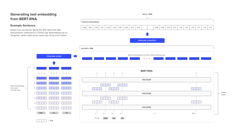
Unlike FinBert, BERT-RNA doesn't have a sentiment classification engine and returns a vector of word embeddings that needs to be further trained on a labeled dataset to perform a classification task. In order to train the classification engine, we need to have a labeled dataset with sentiment scores. For that purpose, I use the same Financial Phrasebook dataset which was used to train the FinBert model.
To do that, I downloaded the dataset from here and stored it in the local directory. Below I read the dataset by replacing sentiment words with labels from 0 to 2.
# read financial phrasebook dataset into a csv
input_df = pd.read_csv('data/sentiment_data/Sentences_50Agree.txt', sep=".@", header=None, encoding="ISO-8859-1", names=['text','label'])
#update the labels
input_df['label'].replace('positive', 0, inplace =True)
input_df['label'].replace('negative', 1, inplace =True)
input_df['label'].replace('neutral', 2, inplace =True)
input_df
| text | label | |
| 0 | According to Gran , the company has no plans t... | 2 |
| 1 | Technopolis plans to develop in stages an area... | 2 |
| 2 | The international electronic industry company ... | 1 |
| 3 | With the new production plant the company woul... | 0 |
| 4 | According to the company 's updated strategy f... | 0 |
| ... | ... | ... |
| 4845 | Sales in Finland decreased by 10.5 % in Januar... | 1 |
4846 rows × 2 columns
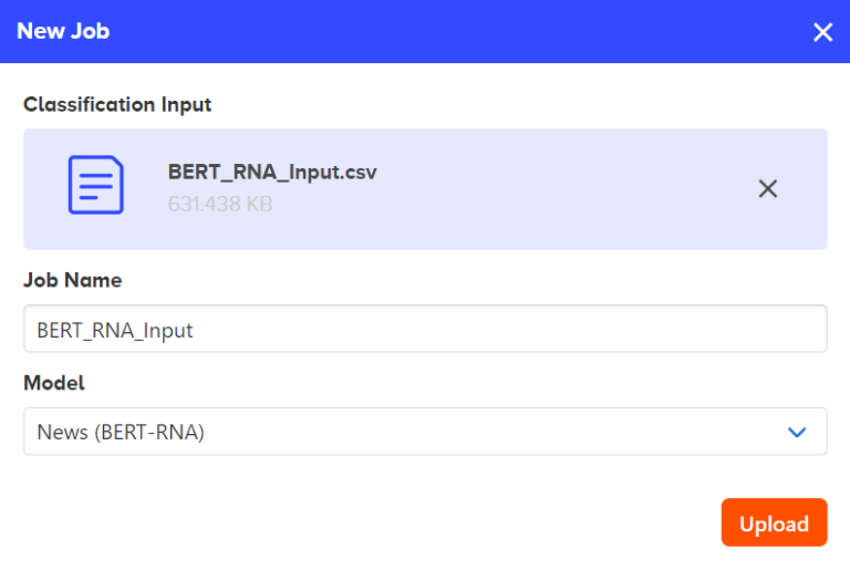
The next step is to format our training data into the CSV structure that BERT RNA accepts. BERT RNA expects a CSV structure with a single column for the text. The header for this column can be named anything.
input_df[['text']].to_csv('BERT_RNA_Input.csv', index=False)
Then I upload the CSV file into the Labs environment by creating a new Job.
After the job is fully executed, an OUT file is created, which can be downloaded from the Labs environment.
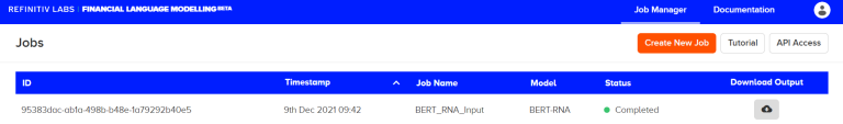
Finally, we can read the out file back to our environment by pandas read_json function.
# read embeddings from .out file exported from the Labs UI
X = pd.read_json('BERT-RNA/data_phrasebook.out')
y = input_df['label']
X
| 0 | 1 | 2 | 3 | 4 | 5 | 6 | 7 | 8 | 9 | ... | 758 | 759 | 760 | 761 | 762 | 763 | 764 | 765 | 766 | 767 | |
| 0 | 0.205987 | -0.972051 | -0.381347 | 0.501484 | 0.447768 | -0.110406 | -0.234994 | 0.848129 | 0.360031 | -0.292546 | ... | 0.913734 | -1.026575 | -0.905293 | -0.347511 | 0.355931 | -0.3144 | -0.214688 | 1.27441 | 0.453175 | -0.341905 |
| 1 | -0.113231 | -0.3017 | 0.002256 | 0.194796 | -0.718617 | -0.341368 | -1.007442 | 0.307653 | 0.209102 | 0.985369 | ... | 0.483089 | -0.847685 | -1.057852 | -1.417513 | 0.23843 | 0.241687 | 0.104607 | 1.550795 | 1.130612 | -0.348374 |
| 2 | -0.684828 | -0.622877 | -0.286472 | 0.148611 | 0.217178 | -0.284424 | -0.645603 | 0.768584 | 0.321413 | 0.908583 | ... | 0.541181 | -0.685226 | -1.008933 | -0.682811 | -0.057627 | 0.381497 | 0.292033 | 1.189711 | 1.192648 | -0.445462 |
| 3 | -0.904132 | 0.030845 | 0.622767 | 0.262248 | 0.077298 | -0.140442 | -0.579286 | 0.101153 | 0.377318 | 0.261287 | ... | 0.56816 | -0.969471 | -0.71147 | -0.391669 | 0.507979 | -0.210143 | 0.211704 | 1.644572 | 0.787941 | -0.044877 |
| 4 | -0.670881 | -0.279356 | 0.123999 | 0.624517 | -0.294081 | 0.547578 | -0.694566 | -0.116304 | 0.309266 | 0.085417 | ... | -0.285442 | -2.091228 | -1.278206 | -0.919836 | 0.67997 | -0.128099 | -0.331344 | 2.467715 | 1.42978 | -0.408402 |
| ... | ... | ... | ... | ... | ... | ... | ... | ... | ... | ... | ... | ... | ... | ... | ... | ... | ... | ... | ... | ... | ... |
| 4845 | -0.612367 | 0.508037 | -0.481639 | -0.288383 | 0.829181 | 1.217645 | -1.065149 | 0.49603 | -0.330197 | -0.392747 | ... | 0.755171 | -1.537933 | -0.021399 | -0.989588 | 0.174585 | 0.040041 | 0.143034 | 2.354939 | 1.13924 | -0.199524 |
4846 rows × 768 columns
The output is a vector for each input token (sentence), and each vector is made up of 768 numbers which correspond to the number of hidden units in the NLP model.
BERT RNA is trained with max sentence length set as 512 tokens. It is advised in BERT-RNA documentation that if the average length of text input is much shorter than 512, the feature space can be very sparse. Thus, applying the dimension reduction technique on the embedding output is recommended.
I will use the Principal component analysis (PCA) technique for dimensionality reduction, but before that, I check the average size of the text inputs.
# get average length of sentences for finding the optimal number of PCA components
length = []
for i in range(len(input_df)):
length.append(len(input_df['text'][i]))
print(f'Average length of our text input is {round(np.mean(length),0)}')
Average length of our text input is 127.0
Now let's apply the PCA dimensionality reduction with principal components of 127.
# run pca
pca = PCA(n_components = 127)
output_pca = pca.fit_transform(X.to_numpy())
Finally, I split PCA output into train and test datasets and run logistic regression to train the sentiment classification model.
#split data into training and testing set
X_train_pca,X_test_pca,y_train_pca,y_test_pca = train_test_split(pd.DataFrame(output_pca), y, test_size = 0.20,random_state=0)
#fit logistic regression model on the training set
logistic_regression_pca = LogisticRegression().fit(X_train_pca,y_train_pca)
#predict labels on testing set and report classification outputs
y_pred_pca = logistic_regression_pca.predict(X_test_pca)
print(classification_report(y_test_pca, y_pred_pca))
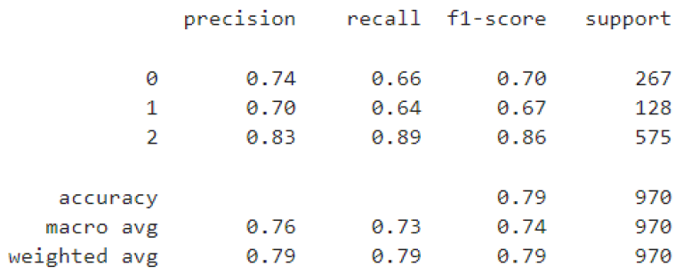
The classification results suggest overall accuracy of 0.79; moreover model produced the highest F1 score on the Neutral class (0.86) and the lowest on the negative class (0.67). The varying accuracy measures can also be caused by the number of instances in each label which is the highest for the neutral (575 instances) and the lowest for the negative class (128 instances).
Overall, the results are satisfactory to proceed with classifying the news sentiment of the target and non-target companies.
Get and Label news headline embeddings from BERT-RNA
First, let's label the news using the BERT-RNA model. For that, I split the news headlines file into 4 different CSVs to make sure the embeddings job is completed properly and download/store the OUT files in a local directory. The code below reads and merges the news headlines into a single dataframe.
# read embeddings from Labs UI exported .out file
sentiment1 = pd.read_json('BERT-RNA/sentiment1.out')
sentiment2 = pd.read_json('BERT-RNA/sentiment2.out')
sentiment3 = pd.read_json('BERT-RNA/sentiment3.out')
sentiment4 = pd.read_json('BERT-RNA/sentiment4.out')
#merge sentiment headlines into one dataframe
sentiment = pd.concat([sentiment1, sentiment2, sentiment3, sentiment4], ignore_index = True, axis = 0)
sentiment
| 0 | 1 | 2 | 3 | 4 | 5 | 6 | 7 | 8 | 9 | ... | 758 | 759 | 760 | 761 | 762 | 763 | 764 | 765 | 766 | 767 | |
| 0 | 0.302118 | -0.395428 | -0.499062 | -0.756795 | 0.039865 | -0.187485 | -0.690534 | -0.056547 | -0.551031 | -1.315916 | ... | -1.288661 | -1.796014 | -0.872499 | -0.292467 | 0.528821 | 0.036952 | -0.718162 | 1.347818 | 0.085477 | 0.36723 |
| 1 | 0.52297 | 0.320371 | 0.283631 | -0.227879 | -0.791052 | -1.029441 | -0.312268 | 0.141227 | -0.785787 | -0.181109 | ... | -0.16645 | -0.972932 | 0.544504 | -0.546426 | 0.284581 | 0.714084 | -0.798771 | 1.70327 | 0.501686 | 0.033989 |
| 2 | 0.5063 | -0.34506 | -0.06983 | 0.214841 | 0.390197 | -0.425927 | 0.368861 | 0.048239 | 0.280302 | -0.359503 | ... | 0.866907 | -1.398539 | -1.72619 | -0.046738 | 1.193358 | 0.838718 | -0.339353 | 0.984092 | 0.768999 | -0.236333 |
| 3 | 0.029535 | 0.541696 | 0.354668 | -0.242215 | -0.471775 | -0.437619 | 0.180205 | 0.6168 | 0.558821 | -0.245121 | ... | 1.109218 | -1.398365 | -0.619977 | -0.273647 | 0.905635 | 0.935657 | -1.365727 | 0.304455 | 0.349801 | -0.232744 |
| 4 | -0.218143 | 0.552087 | 0.342258 | -0.521361 | -0.300859 | -0.641693 | -0.078891 | 0.898205 | 0.515348 | 0.15542 | ... | 0.670583 | -1.259355 | -0.590247 | 0.000672 | 0.545476 | 1.139542 | -1.199727 | 0.049802 | 0.59293 | -0.545367 |
| ... | ... | ... | ... | ... | ... | ... | ... | ... | ... | ... | ... | ... | ... | ... | ... | ... | ... | ... | ... | ... | ... |
| 121966 | -0.06228 | -0.536419 | 0.247584 | -0.161385 | -0.395961 | 0.055131 | -0.544398 | 0.073212 | 0.061124 | 0.042159 | ... | 0.382183 | -1.415708 | -1.149672 | -0.275521 | 0.105553 | 0.545435 | 0.136251 | 0.67413 | 0.689401 | -0.430182 |
121967 rows × 768 columns
Next, I apply PCA dimensionality reduction on our headlines and label them using pre-trained logistic regression model.
#apply dimensionality reduction
sentiment_pca = pca.fit_transform(sentiment.to_numpy())
#predict labels for news headlines
sentL = logistic_regression_pca.predict(sentiment_pca)
#add label list to the headlines dataframe
headlines['sentimentLabs'] = sentL
headlines
| RIC | sdate | edate | Headlines | sentimentLabs | |
| 0 | COR | 16/10/2021 | 10/11/2021 | CIF/FOB Gulf Grain-Corn barge basis steady to ... | 2 |
| 1 | COR | 16/10/2021 | 10/11/2021 | Export Summary-Philippine importer buys feed w... | 2 |
| 2 | COR | 16/10/2021 | 10/11/2021 | PLATTS: 698--Platts Latin America Corn Daily C... | 2 |
| 3 | COR | 16/10/2021 | 10/11/2021 | DJ Thailand Corn Weather - Nov 9 | 2 |
| 4 | COR | 16/10/2021 | 10/11/2021 | DJ Northeast China Corn Weather - Nov 9 | 2 |
| ... | ... | ... | ... | ... | ... |
| 121966 | KNL.N^G21 | 16/08/2020 | 10/09/2020 | COVID-19 Impact & Recovery Analysis | Office F... | 1 |
121967 rows × 5 columns
Label headlines via FinBert model and evaluate pre M&A overall sentiment
Now let's label news headlines via the FinBert model and evaluate pre-M&A overall sentiment by both models. To calculate overall sentiment, I first initiate SentOverallFBert and SentOverallLabs variables starting from 0, and each time a news headline is labeled positive for a particular company, I increase the corresponding variable value by 1 and decrease by 1 if the headline is labeled as negative. Neutral labels don't impact overall sentiment.
Before starting the actual labeling and overall sentiment calculation processes, I first group the news headlines by RICs and then loop over the headlines belonging to the RIC. The code below does the grouping.
dfs = dict(tuple(headlines.groupby('RIC', sort = False)))
Now I loop over each headline of the RIC, label it and calculate overall sentiment for each company based on the two NLP models.
#create empty dictionary to store the sentiment values
sentiments = {'RIC':[],'SentOverallFBert':[],'SentOverallLabs':[]}
#loop over each RIC
for ric in dfs:
#append the RIC to the dictionary
sentiments['RIC'].append(ric)
#initiate overall Sentiment for FinBert
SentOverallFBert = 0
#loop over each news headline belonging to the RIC
for text in dfs[ric]['Headlines']:
#tokenize the headlines
inputs = tokenizer(text, return_tensors="pt")
#get prediction outputs
outputs = model(**inputs)
#get the maximum probability class
sentF = torch.argmax(outputs[0])
#update SentOverallFBert based on the classification output
if sentF == 0:
SentOverallFBert += 1
elif sentF == 1:
SentOverallFBert -= 1
#append FinBert calculated overall sentiment of a company to the dictionary
sentiments['SentOverallFBert'].append(SentOverallFBert)
#initiate overall Sentiment for BERT-RNA
SentOverallLabs = 0
#update SentOverallLabs based on the classification output
for sentL in dfs[ric]['sentimentLabs']:
if sentL == 0:
SentOverallLabs += 1
elif sentL == 1:
SentOverallLabs -= 1
#append BERT-RNA calculated overall sentiment of a company to the dictionary
sentiments['SentOverallLabs'].append(SentOverallLabs)
#convert dictionary to a dataframe
sentiments = pd.DataFrame(sentiments)
Here again, I store the data in an excel file once the code is fully executed and further read from there. The dataset is available in the GitHub folder.
sentiments.to_excel('mergerdata/sentiment_finbert_Labs.xlsx')
#read sentiment dataset from excel
sentiments = pd.read_excel('mergerdata/sentiment_finbert_Labs.xlsx')
Below we plot the overall sentiments calculated by both models to explore the outputs visually and compare the sentiments between the two models.
#plot values using Plotly scatter plot
fig = px.scatter(sentiments, y = ["SentOverallFBert", "SentOverallLabs"])
#update plot layout
fig.update_layout(height=700, width=1100)
fig.update_yaxes(range=[-150, 550], tick0=0)
#move legend to the top left
fig.update_layout(legend=dict(
yanchor="top",
y=0.99,
xanchor="left",
x=0.01
))
fig.show()
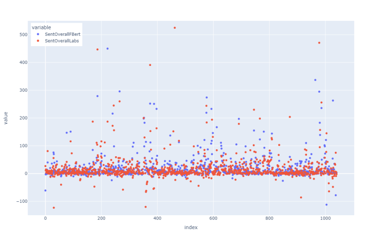
According to the graph, most of the headlines have close to neutral sentiment; moreover, most of the lower negative outputs are classified by BERT-RNA while FinBert has higher positive classifications.
Section 3: Evaluation of M&A predictive modeling
This section evaluates M&A predictive modeling. Before evaluating the ML models, It should be noted that the sample size, especially for the target companies, is very small for robust predictive results. Thus, the primary purpose of this article is to showcase a workflow of M&A predictive modeling using Refinitiv data/APIs and discover if news sentiment has any significant explanatory impact on the predictive power of the model. And, if one wants to build a robust M&A predictive model can use this workflow and variables to train the models on much larger datasets.
Logistic regression, random forests, and XGBoost ML techniques are used for the predictive modeling. The reason for using multiple ML techniques is to evaluate the explanatory power of news sentiment variables from multiple perspectives and make a robust conclusion regarding the importance of that variable on the M&A predictive modeling. Particularly, logistic regression allows looking at the p-values and the coefficients of the variables and random forest and XGBoost evaluate the importance of the features.
As these models are not used for actual prediction but rather for showing the impact of the sentiment variables on evaluation metrics, instead of train/test split, I employ Repeated Stratified Cross-Validation with 10 splits and 5 repeats. Considering the imbalanced nature of the dataset, ROC_AUC score is used as the main accuracy metric.
#set index columns to implement dataframe joining
all_data.set_index('Instrument', inplace = True)
sentiments.rename(columns = {"RIC": "Instrument"}, inplace=True)
sentiments.set_index('Instrument', inplace = True)
#join NLP based and financial variable datasets
all_data = all_data.join(sentiments, on = 'Instrument', how = 'inner').reset_index().drop_duplicates(subset = ['Instrument'], keep = 'first')
all_data.head()
| Instrument | AD | Gross Profit Margin - % | Operating Margin - %, TTM | Current Ratio | Price To Book Value Per Share (Daily Time Series Ratio) | Price To Sales Per Share (Daily Time Series Ratio) | Net Debt per Share | Label | Profit to Capital | Free Cash Flow to Sales | Cash to Capital | EV to EBITDA | Debt to EV | AR | Sales_growth | SentOverallFBert | SentOverallLabs | |
| 0 | COR | 15/11/2021 | 40.21891 | 22.855325 | 0.39338 | 320.578875 | 9.957096 | 39.991626 | 1 | 0.044347 | 0.005647 | 0.003099 | 51.388454 | 0.214218 | -0.858267 | 8.048231 | -61 | 27 |
| 1 | DVD | 09/11/2021 | 26.66113 | 25.492173 | 3.47706 | 1.068976 | 1.019694 | -0.345537 | 1 | 0.108392 | 0.031004 | 0.182074 | 12.643395 | 0 | -11.662717 | -5.932295 | -3 | 11 |
| 2 | MCFE.O | 08/11/2021 | 62.31934 | 10.883691 | 0.38323 | -0.979807 | 4.451983 | 8.768888 | 1 | -0.053955 | 0.247075 | 0.105624 | 28.844474 | 0.194682 | -12.960495 | 11.902193 | 1 | 15 |
| 3 | CPLG.K | 08/11/2021 | -10.7056 | -30.140187 | 4.58824 | 1.060099 | 2.12139 | 11.758621 | 1 | -0.105826 | -0.150852 | 0.085018 | -116.99623 | 0.587626 | 12.219687 | -17.358218 | -2 | 3 |
| 4 | MNR | 05/11/2021 | 81.96786 | 49.471649 | 11.5161 | 1.641761 | 10.420573 | 8.678789 | 1 | -0.01158 | -0.491178 | 0.012299 | 39.203266 | 0.262022 | -0.604319 | 13.026745 | -2 | 5 |
| ... | ... | ... | ... | ... | ... | ... | ... | ... | ... | ... | ... | ... | ... | ... | ... | ... | ... | ... |
| 1309 | KNL.N^G21 | 15/09/2020 | 38.44269 | 7.734148 | 1.17448 | 1.691853 | 0.510063 | 8.789553 | 0 | 0.077266 | 0.06183 | 0.00973 | 6.547313 | 0.385728 | 0.338345 | 8.204436 | 3 | -2 |
1031 rows × 18 columns
Then I run correlation analysis to eliminate the highly correlated variables and avoid multicollinearity. The code below unstacks and sorts the outputs showing the highly correlated variables.
all_data.corr().unstack().sort_values().drop_duplicates()
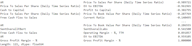
It can be observed from the correlation output that Abnormal return(AR) is correlated with Price To Sales Per Share and EV to EBITDA. At the same time, the latter two variables are highly correlated with each other as well. Thus, I removed both of them and kept AR for the final model. Another correlated pair is Free Cash Flow to Sales and Operating Margin. Among those, I eliminated operating margin since there is already another variable, Gross Profit Margin, describing the management efficiency component of the company.
I drop the variables Operating Margin, EV to EBITDA, and Price to Sales per Share in the cell below. Additionally, I created three different sets of independent variables. The first dataset (X_NoSent) consists of only financial variables, the second dataset (X_BertRna) includes the overall sentiment variable derived by the BERT-RNA model, and the third one (X_Finbert) includes overall sentiment based on the FinBert model. Throughout the analysis, evaluation metrics based on all three datasets are reported to showcase the effect of news sentiment variable, including in relation to AR.
#drop correlated variables
X = all_data.drop(columns = ['Instrument', 'Label', 'AD', 'Operating Margin - %, TTM','EV to EBITDA',
'Price To Sales Per Share (Daily Time Series Ratio)'])
y = all_data['Label']
#create separate datasets for no sentiment and sentiment based data
X_NoSent = X.drop(columns = ['SentOverallLabs', 'SentOverallFBert'])
X_BertRna = X.drop(columns = ['SentOverallFBert'])
X_Finbert = X.drop(columns = ['SentOverallLabs'])
3.2 Evaluation of Logistic regression model outputs
First, I train and evaluate the outputs from the logistic regression with a 'liblinear solver' and the penalty of 'l2'. This will allow us to look at p-values and coefficients of the independent variables helping to make certain conclusions regarding the impact of the sentiment variables. As the main accuracy metric the ROC_AUC score is used.
#initiate logistic regression model
lr = LogisticRegression(solver = 'liblinear', penalty = 'l2', random_state = 0)
#define cross validation parameters
cv = RepeatedStratifiedKFold(n_splits = 20, n_repeats = 5, random_state = 0)
#run cross validation on logistic regression model with defined CV parameters
scoresNoSent = cross_validate(lr, X_NoSent, y, scoring=['roc_auc'], cv = cv, n_jobs = -1)
scoresBertRna = cross_validate(lr, X_BertRna, y, scoring=['roc_auc'], cv = cv, n_jobs = -1)
scoresFinbert = cross_validate(lr, X_Finbert, y, scoring=['roc_auc'], cv = cv, n_jobs = -1)
#report cross validation outputs on 3 datasets
print('\033[1m' + "Model with no sentiment variable" + '\033[0m')
print("AUC:" + str(round(scoresNoSent['test_roc_auc'].mean(),2)))
print('\033[1m' + "With Sentiment from BERT-RNA" + '\033[0m')
print("AUC:" + str(round(scoresBertRna['test_roc_auc'].mean(),2)))
print('\033[1m' + "With Sentiment from FinBert" + '\033[0m')
print("AUC:" + str(round(scoresFinbert['test_roc_auc'].mean(),2)))
Model with no sentiment variable
AUC:0.5
With Sentiment from BERT-RNA
AUC:0.54
With Sentiment from FinBert
AUC:0.57
From the reported ROC_AUC scores, we can clearly see that logistic regression models with NLP-based sentiment variable significantly outperform the no sentiment model. Moreover, the model with sentiment derived by the FinBert model achieves the highest accuracy of 0.57. Further, I calculate and report coefficients and p-values of variables from the FinBert sentiment-based model. This will show the significance and the direction of the impact of the variables. For that, I first normalize the data by subtracting the mean from the actual values and dividing the outcome by the standard deviation. This will normalize the data and make sure the explainability of the coefficients.
#normalize the data
X_norm = (X_Finbert - np.mean(X_Finbert)) / np.std(X_Finbert, 0)
#fit logistic regression model with normalized data
model = lr.fit(X_norm, y)
#create a dataframe consisting of the list of coefficients
coefs = pd.DataFrame(index = X_Finbert.columns, data = model.coef_[0], columns = ['Coefficients'])
Before showing the resulting dataframe of coefficients, I add to that the p-values for a more comprehensive outlook. As known, sklearn doesn't have a built-in package for p-value calculation; thus, I calculate it myself by adapting an example from a thread in Stackoverflow.
def logit_pvalue(model, x):
'''
Calculate z-scores for scikit-learn LogisticRegression.This function uses asymtptics for maximum likelihood estimates.
Parameters:
------------
Input
model: fitted sklearn.linear_model.LogisticRegression with intercept and large C
x: matrix on which the model was fit
Output:
p: array of p-values
'''
p = model.predict_proba(x)
n = len(p)
m = len(model.coef_[0]) + 1
coefs = np.concatenate([model.intercept_, model.coef_[0]])
x_full = np.matrix(np.insert(np.array(x), 0, 1, axis = 1))
ans = np.zeros((m, m))
for i in range(n):
ans = ans + np.dot(np.transpose(x_full[i, :]), x_full[i, :]) * p[i,1] * p[i, 0]
vcov = np.linalg.inv(np.matrix(ans))
se = np.sqrt(np.diag(vcov))
t = coefs/se
p = (1 - norm.cdf(abs(t))) * 2
return p
#get p-values
zScores = logit_pvalue(model, X_Finbert)
#convert from scientific numpers
zScores = ['{0:f}'.format(num) for num in zScores][1:]
#append p-values to coefficient's dataframe
coefs.insert(loc = len(coefs.columns), column = 'P-Value', value = zScores)
coefs.T
| Gross Profit Margin - % | Current Ratio | Price To Book Value Per Share (Daily Time Series Ratio) | Net Debt per Share | Profit to Capital | Free Cash Flow to Sales | Cash to Capital | Debt to EV | AR | Sales_growth | SentOverallFBert | |
| Coefficients | -0.038679 | -0.001491 | 0.096708 | -0.44698 | 0.019854 | 0.075284 | 0.013539 | -0.046934 | 0.531696 | 0.093291 | -0.45572 |
| P-Value | 0.000125 | 0.991442 | 0.000069 | 0 | 0.966635 | 0.899132 | 0.987717 | 0.961843 | 0 | 0 | 0 |
From the results above, we can observe a statistically significant impact of Gross Profit Margin, Price To Book Value Per Share, Net Debt per Share, AR, Sales Growth, and SentOverallFBert variables. Moreover, the coefficient of SentOverallFBert is one of the biggest and equals to -0.46. At the same time, the coefficient of AR is the biggest equalling to 0.53. The negative coefficient of SentOverallFBert and the positive coefficient of AR (both statistically significant) suggest that higher abnormal return and lower positive sentiment indicate a higher possibility of M&A. This is in line with my initial assumption and supports the hypothesis that abnormal returns amid no or lower positive news is an indication of M&A announcement.
Further, I train and evaluate random forest and XGBoost models on the same datasets and look at the differences of the evaluation metrics across the models with different datasets. Most importantly, I look at the feature importance to confirm the significance of the Sentiment variable for the M&A predictive modeling.
3.3 Evaluation of Random forest model outputs
Next, I train and evaluate the outputs from the random forest model with 500 estimators and the entropy criterion. I used balanced subsample class weight considering the imbalanced nature of the dataset. Also, I set the value of the parameter max_depth to 3 to make sure I don't overfit the model. ROC_AUC score is used as the main accuracy metric. Additionally, I report values for precision, recall, and F1. Finally, I look at the feature importance of independent variables to evaluate the significance of sentiment variables according to the random forest model.
#initiate random forest model with specified parameters
rf = RandomForestClassifier(n_estimators=500, class_weight='balanced_subsample', criterion='entropy', max_depth = 3, n_jobs=-1, random_state = 5)
#run cross validation on random forest model with defined CV parameters
scoresNoSentRf = cross_validate(rf, X_NoSent, y, scoring = ['roc_auc', 'accuracy', 'f1', 'precision', 'recall'], cv = cv, n_jobs = -1)
scoresBertRnaRf = cross_validate(rf, X_BertRna, y, scoring = ['roc_auc', 'accuracy', 'f1', 'precision', 'recall'], cv = cv, n_jobs = -1)
scoresFinbertRf = cross_validate(rf, X_Finbert, y, scoring = ['roc_auc', 'accuracy', 'f1', 'precision', 'recall'], cv = cv, n_jobs = -1)
#report cross validation outputs on 3 datasets
print('\033[1m' + "Model with no sentiment variable" + '\033[0m')
print("AUC:" + str(round(scoresNoSentRf['test_roc_auc'].mean(),2)))
print("Precision:" + str(round(scoresNoSentRf['test_precision'].mean(),2)))
print("Recall:" + str(round(scoresNoSentRf['test_recall'].mean(),2)))
print("F1:" + str(round(scoresNoSentRf['test_f1'].mean(),2)))
print('\033[1m' + "With Sentiment from BERT-RNA" + '\033[0m')
print("AUC:" + str(round(scoresBertRnaRf['test_roc_auc'].mean(),2)))
print("Precision:" + str(round(scoresBertRnaRf['test_precision'].mean(),2)))
print("Recall:" + str(round(scoresBertRnaRf['test_recall'].mean(),2)))
print("F1:" + str(round(scoresBertRnaRf['test_f1'].mean(),2)))
print('\033[1m' + "With Sentiment from FinBert" + '\033[0m')
print("AUC:" + str(round(scoresFinbertRf['test_roc_auc'].mean(),2)))
print("Precision:" + str(round(scoresFinbertRf['test_precision'].mean(),2)))
print("Recall:" + str(round(scoresFinbertRf['test_recall'].mean(),2)))
print("F1:" + str(round(scoresFinbertRf['test_f1'].mean(),2)))
Model with no sentiment variable
AUC: 0.62
Precision: 0.24
Recall: 0.49
F1: 0.32
With Sentiment from BERT-RNA
AUC: 0.64
Precision: 0.25
Recall: 0.49
F1: 0.33
With Sentiment from FinBert
AUC: 0.64
Precision: 0.26
Recall: 0.51
F1: 0.34
Reported evaluation metrics are in line with the one from the logistic regression model in terms of models with NLP-based sentiment variable outperforming the no sentiment model. Moreover, we observe a much higher ROC_AUC score for random forest models. Particularly, it is 0.12 higher for the no sentiment variable model and 0.11, 0.7 higher for models with sentiments from BERT_RNA and FinBert sentiment, respectively. It is worth also highlighting that FinBert and BERT_RNA based models have the same ROC_AUC score of 0.64; however, FinBert still slightly outperforms BERT_RNA by precision, recall, and F1 measures.
Next, I calculate and plot the feature importance for both models with sentiment variables.
#calculate feature importance
importanceFinbertRf = [round(imp,2) for imp in rf.fit(X_Finbert, y).feature_importances_]
importanceBertRnaRf = [round(imp,2) for imp in rf.fit(X_BertRna, y).feature_importances_]
#create subplots for two models
fig = make_subplots(
rows=2, cols=1, subplot_titles=[
'Feature importance for model with FinBert Sentiment',
'Feature importance for model with BERT-RNA Sentiment'])
#add barplot for feature importance from FinBert model
fig.add_trace(go.Bar(y = X_Finbert.columns, x = importanceFinbertRf,
orientation='h', text = importanceFinbertRf, showlegend = False), row=1, col=1)
#add barplot for feature importance from BERT_RNA model
fig.add_trace(go.Bar(y = X_BertRna.columns, x = importanceBertRnaRf,
orientation='h', text = importanceBertRnaRf, showlegend = False), row=2, col=1)
#update layout and sort values inside the plot
fig.update_layout(height = 800, width = 1100)
fig.update_yaxes(categoryorder='total ascending')
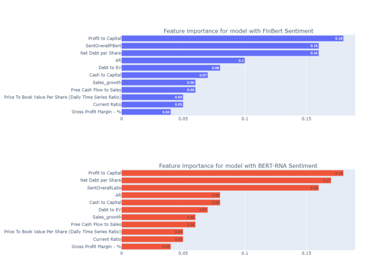
Both of the graphs above suggest the high importance of the news sentiment variable. Particularly, SentOverallFBert has the second-highest feature importance after Profit to Capital. The latter has the highest importance in the model based on BERT_RNA as well. In that model, Net Dept per Share has slightly higher importance than SentOverallLabs. Nevertheless, the results from the feature importance values are in line with the results from the logistic regression model. They show the high importance of NLP-based news sentiment variables along with AR variable.
3.4 Evaluation of XGBoost model outputs
Finally, I train and evaluate the outputs from the XGBoost model with 500 estimators, a learning rate of 0.1, and an alpha of 30. I used the balanced scale_pos_weihght parameter considering the imbalanced nature of the dataset. Also, I set the parameter max_depth to 3 and subsample to 0.5 to make sure I don't overfit the model. Here again, the ROC_AUC score is used as the main accuracy metric. Additionally, I report values for precision, recall, and F1. Finally, I look at the feature importance of independent variables to evaluate the significance of sentiment variables according to the XGBoost model.
#calculate number of target and non-target companies for assigning weights
target = all_data[all_data['Label'] == 1].shape[0]
nontarget = all_data[all_data['Label'] == 0].shape[0]
#initiate XGBoost model with specified parameters
xgBoost = XGBClassifier(scale_pos_weight = nontarget/target, max_depth=3, subsample = 0.5, n_estimators = 500, learning_rate = 0.1, alpha = 30)
#run cross validation on XGBoost model with defined CV parameters
scoresNoSentXgb = cross_validate(xgBoost, X_NoSent, y, scoring = ['roc_auc', 'accuracy', 'f1', 'precision', 'recall'], cv = cv, n_jobs = -1)
scoresBertRnaXgb = cross_validate(xgBoost, X_BertRna, y, scoring = ['roc_auc', 'accuracy', 'f1', 'precision', 'recall'], cv = cv, n_jobs = -1)
scoresFinbertXgb = cross_validate(xgBoost, X_Finbert, y, scoring = ['roc_auc', 'accuracy', 'f1', 'precision', 'recall'], cv = cv, n_jobs = -1)
#report cross validation outputs on 3 datasets
print('\033[1m' + "Model with no sentiment variable" + '\033[0m')
print("AUC:" + str(round(scoresNoSentXgb['test_roc_auc'].mean(),2)))
print("Precision:" + str(round(scoresNoSentXgb['test_precision'].mean(),2)))
print("Recall:" + str(round(scoresNoSentXgb['test_recall'].mean(),2)))
print("F1:" + str(round(scoresNoSentXgb['test_f1'].mean(),2)))
print('\033[1m' + "With Sentiment from BERT-RNA" + '\033[0m')
print("AUC:" + str(round(scoresBertRnaXgb['test_roc_auc'].mean(),2)))
print("Precision:" + str(round(scoresBertRnaXgb['test_precision'].mean(),2)))
print("Recall:" + str(round(scoresBertRnaXgb['test_recall'].mean(),2)))
print("F1:" + str(round(scoresBertRnaXgb['test_f1'].mean(),2)))
print('\033[1m' + "With Sentiment from FinBert" + '\033[0m')
print("AUC:" + str(round(scoresFinbertXgb['test_roc_auc'].mean(),2)))
print("Precision:" + str(round(scoresFinbertXgb['test_precision'].mean(),2)))
print("Recall:" + str(round(scoresFinbertXgb['test_recall'].mean(),2)))
print("F1:" + str(round(scoresFinbertXgb['test_f1'].mean(),2)))
Model with no sentiment variable
AUC: 0.62
Precision: 0.24
Recall: 0.48
F1: 0.32
With Sentiment from BERT-RNA
AUC: 0.63
Precision: 0.25
Recall: 0.49
F1: 0.33
With Sentiment from FinBert
AUC: 0.64
Precision: 0.26
Recall: 0.53
F1: 0.35
Reported evaluation metrics are in line with the one from the random forest model. Here again, we observe a much higher ROC_AUC score compared to the logistic regression outputs. It is worth also highlighting that here FinBert based model still slightly outperforms the BERT_RNA-based one not only by precision, recall, and F1 measures but also on the ROC_AUC score.
Here again, I calculate and plot the feature importance for both models with sentiment variables.
importanceFinbertXgb = [round(imp,2) for imp in xgBoost.fit(X_Finbert, y).feature_importances_]
importanceBertRnaXgb = [round(imp,2) for imp in xgBoost.fit(X_BertRna, y).feature_importances_]
fig = make_subplots(
rows=2, cols=1, subplot_titles=[
'Feature importance for model with FinBert Sentiment',
'Feature importance for model with BERT-RNA Sentiment'])
fig.add_trace(go.Bar(y = X_Finbert.columns, x = importanceFinbertXgb,
orientation='h', text = importanceFinbertXgb, showlegend = False), row=1, col=1)
fig.add_trace(go.Bar(y = X_BertRna.columns, x = importanceBertRnaXgb,
orientation='h', text = importanceBertRnaXgb, showlegend = False), row=2, col=1)
fig.update_layout(height=800, width=1100)
fig.update_yaxes(categoryorder='total ascending')
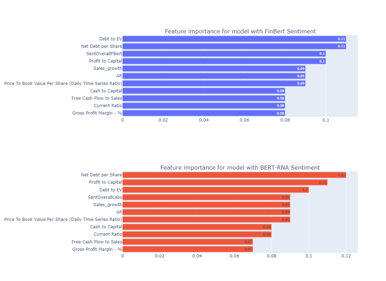
As in the case of the random forest model, both of the graphs suggest that the news sentiment variable is among the highest important features. The main distinctive part of XGBoost feature importance is that it revealed Debt to EV as another important feature which value exceeds both SentOverallFBert and SentOverallLabs. Nevertheless, the results from feature importance values are in line with the results from the logistic regression model and the random forest models suggesting the high importance of NLP-based news sentiment variables.
Summary
This article was an extension to my first article on Predicting M&A targets using Machine Learning techniques. If the first article used only financial variables to predict M&A, here the NLP-based news sentiment variable was used to increase the predictive power of the model. The main hypothesis behind the news sentiment variable was the intuition that abnormal returns amid no or lower positive news sentiment environment could indicate an M&A announcement. For the news sentiment analysis, two BERT-based models, including FinBert and BERT-RNA, are used and the significance of variables derived by both of the models through logistic regression, random forest, and XGBoost ML techniques, are compared.
Although the dataset wasn't large enough to claim the robustness of the model's predictive power, the evaluation results on different ML techniques allow to claim the importance of the NLP-based news sentiment variable along with Abnormal return for the M&A predictive analysis. In fact, the latter was the main purpose of this article. Although the predictive power of this model isn't high enough to use this model for an actual prediction and trading, I hope that this prediction workflow along with the selected variables, can be useful for training more robust models on much larger datasets and achieve much higher accuracies.
Apart from this, another important aspect of this article was the usage of the Search function for M&A data retrieval and the usage of BERT-RNA embeddings for sentiment classification, which I believe can be useful for the developer community who use Refinitv products.