


Applications of Generative Adversarial Networks
Data can sometimes be difficult to find or expensive and time-consuming to acquire. Furthermore, data can be sensitive and difficult to share. In such situations, Generative Adversarial Networks (GAN)s can be a valuable tool. Artificially recreating a dataset is a complex and sensitive process. The new data need to correctly mimic the existing data distributions and not introduce biasing or noise in the dataset. GANs can uncover the deeper structure of a small dataset to create an infinite amount of new data. GANs contribute to financial innovation as the technique allows us to:
· Explore strategic collaborations: When sensitive data cannot be shared and in circumstances where even anonymization is not enough generating a new dataset mimicking the existing one allows us to distribute it without the possibility of a reverse trace.
· Create data that we do not have: We can pretty much create an unlimited amount of data thereby not constraining ourselves in the data that exists. This, especially in the context of a data hungry deep learning algorithm can be quite important. We can furthermore enhance existing datasets with external dataset distribution and increase the predictive value of the data.
The technique
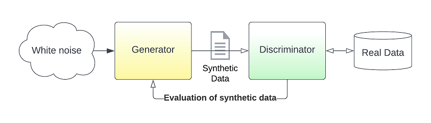
A GAN is a complex twin neural network structure that tries to learn the data and then generates new data from it. We call it a twin structure as it is comprised of the Generator and the Discriminator neural networks that are competing each other during learning. The learning process mimics the way we as humans learn with the help of an expert. We try to solve a problem succeed or fail but nonetheless we receive feedback from the expert on what to do better next time we try. In that exact same way, the Generator NN starts by knowing nothing about the data and receiving noise as an input, the latent space, can only generate pure noise. After every attempt to generate data, the discriminator, which is an expert in the data, will mark the attempt from 0 to 1 depending on how realistic the data looks. The generator will try again and again until the discriminator is convinced that the data presented belongs to the dataset it knows. At that point the Generator is now an expert on the data even though it has never seen the data and can generate an infinite amount of data.
Important notes
As a GAN is a complex technique there can be a few problems with its applications, they fall into three main categories:
- Mode collapse: Sometimes the distribution of the dataset is too complex, and the GAN may fail to best capture it. In a multi-modal probability distribution, the GAN may learn a single dominant mode of the data. If this is the case, we can use ensemble GAN structures or use data sampling to improve results.
- Vanishing gradients: As can be the case with all Neural Networks, during back-propagation, as the gradient flows backwards, it can get so small that it does not alter the weights of the network. This problem can become more prominent as we increase the depth of the Neural Network. To overcome the problem try using different activation functions such as ReLU, LeakyReLU and PReLU.
- Stability and convergence issues: For some datasets the generator and discriminator may never reach a satisfying solution. Several techniques can be introduced to overcome the matter including feature matching, mini batch discrimination, historical averaging, batch normalisation and more.
Other Variants
WGAN, DCGAN, StackGAN, CycleGAN, 3DGAN, TimeGAN
Blueprint - Generating flash crash data
In this blueprint on Tensorflow we will implement a base GAN structure which we will then use to generate synthetic data from the event of a market flash crash. This is a candidate use case for the AI structure as such events last for a very short time and may not generate enough data for analysis purposes. Quite recently we have witnessed such an event on the Stockholm Stock Exchange, we will be ingesting OMX index futures tick data using Refinitiv Data libraries in an effort to generate the synthetic dataset that will follow the event distribution.
Ingesting tick data using RD libraries is as simple as a few sequential rd.get_history() calls with the correct time frames as parameters to create a continuous stream of tick data. The reason for the use of the while loop and dates methodology is the 10000 data points cap per call on RD processes, a cap that is sufficient for most scenarios but that can be easily reached in the tick data space.
def get_tick_data(instrument, start_date, end_date):
df = pd.DataFrame()
end_date = parser.parse(end_date).replace(tzinfo=None)
start_date = parser.parse(start_date).replace(tzinfo=None)
print(f'Requesting tick data for {instrument} for the period {start_date} to {end_date}')
while end_date >= start_date:
try:
temp_df = rd.get_history(universe=[instrument],
end=end_date, count=5000,
fields=["BID", "ASK", "EVENT_TYPE", "BIDSIZE", "ASKSIZE","TRDPRC_1","TRDVOL_1", "VWAP", "ACVOL_UNS", "RTL", "SEQNUM"],interval='tick')
end_date=temp_df.index.min().replace(tzinfo=None).strftime('%Y/%m/%d%H:%M:%S.%f')
end_date = datetime.strptime(end_date, '%Y/%m/%d%H:%M:%S.%f')
if len(df):
df = pd.concat([df, temp_df], axis=0)
else:
df = temp_df
except:
continue
df.reset_index(inplace=True)
df['BID'] = pd.to_numeric(df['BID'])
df['ASK'] = pd.to_numeric(df['ASK'])
df['BIDSIZE'] = pd.to_numeric(df['BIDSIZE'])
df['ASKSIZE'] = pd.to_numeric(df['ASKSIZE'])
df['TRDVOL_1'] = pd.to_numeric(df['TRDVOL_1'])
df['TRDPRC_1'] = pd.to_numeric(df['TRDPRC_1'])
df['VWAP'] = pd.to_numeric(df['VWAP'])
df['ACVOL_UNS'] = pd.to_numeric(df['ACVOL_UNS'])
df['RTL'] = pd.to_numeric(df['RTL'])
df['SEQNUM'] = pd.to_numeric(df['SEQNUM'])
print(f'{df.shape[0]} datapoints for {instrument} are created and stored')
return df
Once we have downloaded the data we can save the dataframe into a csv file. Let's now load the data and generate a few base features from the existing ones. The following code segment, part of the feature engineering stage creates TPT which is the rate of trades per tick and PRICE_GRADIENT which is easily calculated using the tick_gradient() function:
def tick_gradient(start_tick, end_tick, start_prx, end_prx):
return (end_prx - start_prx)/(end_tick - start_tick)
def read_de_output():
df = pd.read_csv(data_file_path)
df = df.sort_values(by='Timestamp')
df = df[df['Timestamp'] >= '2022-05-02 07:00:00.000000+00:00']
df['SEQNUM'] = range(1, df.shape[0] + 1)
trade_tick_data = df[df['EVENT_TYPE'] == 'trade']
trade_tick_data = trade_tick_data[['Timestamp',
'SEQNUM',
'TRDPRC_1',
'TRDVOL_1']]
trade_tick_data['TNO'] = range(1, trade_tick_data.shape[0] + 1)
trade_tick_data['TPT'] = trade_tick_data['TNO'] / trade_tick_data['SEQNUM']
price_gradient = [0]
for i in range(1, trade_tick_data.shape[0]):
price_gradient.append(np.abs(tick_gradient(trade_tick_data.iloc[i- 1, 1],
trade_tick_data.iloc[i, 1],
trade_tick_data.iloc[i-1, 2],
trade_tick_data.iloc[i, 2])))
trade_tick_data['PRICE_GRADIENT'] = price_gradient
trade_tick_data = trade_tick_data.set_index('Timestamp')
return trade_tick_data
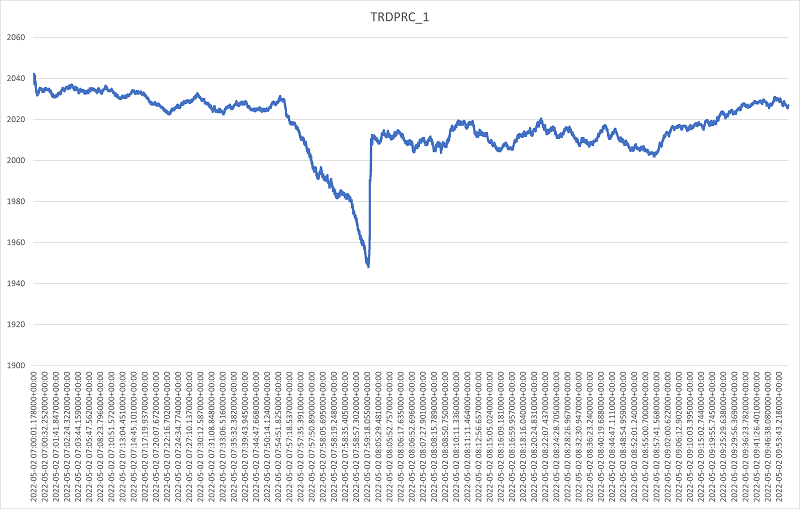
Let's now plot all the tick trade events prices to get a visual representation of the flash crash.
We then plot the corresponding tick data trade price gradients, essentially this depicts the trade price velocity. We use absolute values as we are interested in the velocity rather than the direction of change.
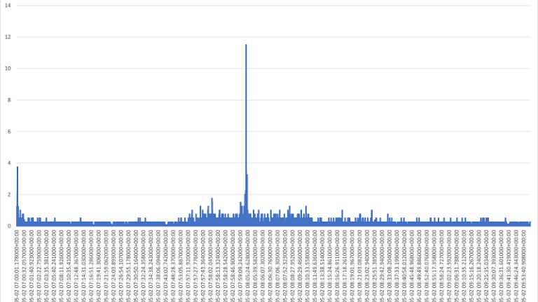
As expected we see an increase in the absolute gradient of the price as we approach the region of the flash crash event around 9:55am and a sharp increase at the moment the market reacts in an effort to absorb the event at around 10:05am. Thereafter, the gradient remains high as further oscillations are propagated in the market and returns closer to normality after 10:30m. Assuming that we would like to be working on this simplified feature space to model market microstructure during the event, as a first step let's roughly filter the event at 9:55am to 10:05am.
fc_trade_tick_data = trade_tick_data.loc['2022-05-02 07:55:00.000000+00:00':'2022-05-02 08:05:00.000000+00:00', :]
Next step is the main feature engineering part, we scale the data using the StandardScaler and apply a 2 components PCA to achieve compression and to allow us to visualise results for the purposes of the article. Notice that the function aside from returning the resulting matrices also pickles the output into binary compressed files that can be loaded later at the next phase of the pipeline. This would allow for a more productionised style pipeline.
def transform_real_sample(df):
scaler_file = 'scaler.pickle'
pca_file = 'pca.pickle'
X = df.to_numpy()
scaler = StandardScaler()
X_scaled = scaler.fit_transform(X)
pca_model = PCA(n_components=2)
x_pca = pca_model.fit_transform(X_scaled)
with open(scaler_file, 'wb') as f:
pickle.dump(scaler, f, protocol=pickle.HIGHEST_PROTOCOL)
with open(pca_file, 'wb') as f:
pickle.dump(pca_model, f, protocol=pickle.HIGHEST_PROTOCOL)
c = np.ones(df.shape[0]).reshape(df.shape[0], 1)
return x_pca, c
Modelling the Generative Adversarial Network
As we mentioned a GAN is comprised of a Discriminator and a Generator Neural Network. Remember that only the Discriminator knows about the actual data. The generator starts by seeing pure noise and tries to move the distribution in such a way that the Discriminator will be fooled that it belongs to the distribution it already knows. Let's define the two separate Model structures and combine them together in a competing GAN structure:
from tensorflow.keras.models import Sequential
from tensorflow.keras.layers import Dense
def discriminator_model(input_dimensions=2):
model = Sequential()
model.add(Dense(10, activation='relu', input_dim=input_dimensions))
model.add(Dense(1, activation='sigmoid'))
model.compile(loss='binary_crossentropy', optimiser='adam', metrics=['accuracy'])
return model
def generator_model(input_dimensions=2, output_dimensions=2):
model = Sequential()
model.add(Dense(10, activation='relu', input_dim=input_dimensions))
model.add(Dense(output_dimensions, activation='linear'))
return model
def GAN(discriminator, generator):
discriminator.trainable=False
model = Sequential()
model.add(generator)
model.add(discriminator)
model.compile(loss='binary_crossentropy', optimiser='adam')
return model
Now let’s create a helper function, that generates pure noise:
def noise(dimensions, n):
return randn(dimensions*n).reshape(n, dimensions)
We will use the generator to create a synthetic sample:
def get_synthetic_sample(generator: Sequential, noise_dimensions, n):
x = noise(noise_dimensions, n)
X = generator.predict(x)
c = np.zeros(n).reshape(n, 1)
return X, c
We can now train the GAN structure:
def train(generator: Sequential, discriminator: Sequential, gan: Sequential, noise_dimensions, epochs=2000, batch_size=64):
for i in range(epochs):
x_actual, y_actual = get_polynomial_sample(batch_size)
x_synthetic, y_synthetic = get_synthetic_sample(generator, noise_dimensions, batch_size)
discriminator.train_on_batch(x_actual, y_actual)
discriminator.train_on_batch(x_synthetic, y_synthetic)
x_gan = noise(noise_dimensions, batch_size)
y_gan = np.ones((batch_size, 1))
gan.train_on_batch(x_gan, y_gan)
epoch_results(i, generator, discriminator, noise_dimensions, batch_size)
Finally, to kickoff everything we write the following main function:
if __name__ == '__main__':
noise_dimensions = 3
generator = generator_model(noise_dimensions)
discriminator = discriminator_model()
gan = GAN(discriminator, generator)
train(generator, discriminator, gan, noise_dimensions)
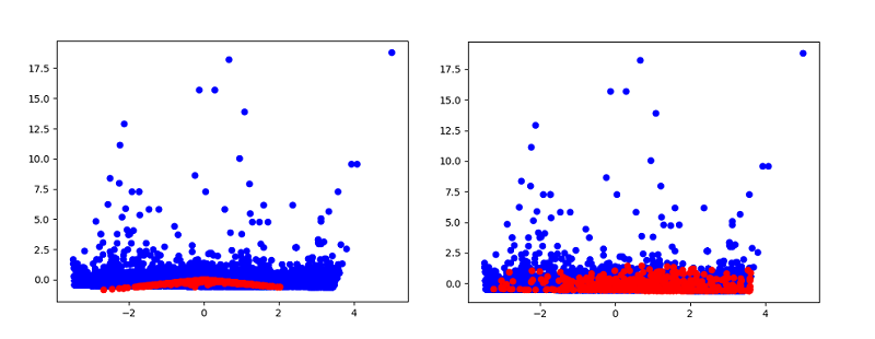
We trained the structure for 90.000 epochs. The diagrams below show the results on the first epoch and the 90.000 epoch. The blue points are the actual main principal components describing the flash crash baseline microstructure as we have defined it in the previous sections of the article. The red points are the newly generated data starting from noise. We can see that after the 90.000 epoch the generated data fairly mimic the actual data distribution. In essence we have doubled the amount of data we have on the flash crash.
Conclusions
In this article we used a Generative Adversarial Network to generate synthetic data based on a flash crash event. Despite the fact that this methodology entails a full pipeline, we attribute it to the feature engineering phase as we focus on generating more data that will represent the event. In an article to follow we will focus on the modelling and evaluation phase of the methodology and the steps that need to be taken to ensure an optimised training process. For example our topology here is very basic, e.g. only a single 10 neuron layer, which may not be able to capture all of the variance present in the event. We can see this from the 90000 epoch output where we have a good fit for the base, but no real attempt to recreate the outlier data points with any success. After the enhanced modelling and evaluation process we can try to use the newly created data to recreate a flash crash and explore the possibility of implementing an early detection process.