
Author:

Overview
This article will introduce a simple approach to begin to model energy markets. In our case we will be looking to see if we can ascertain any impact on German energy prices when the wind blows. Energy markets are quite complex to model nevertheless we will try to have a go at this using some of the tools available in the Python scientific computing ecosystem. I hope to demonstrate that it is possible with a little effort.
We will be using a mix of data from different sources combined with data from both Eikon and the Refinitiv Data Platform as well as our Point Connect service. We will be using some APIs and also some file-based sources. I will include any data files in the code repository so you can replicate.
Sections
Locating Weather Monitoring Stations
Calculate nearest weather station for each windfarm
Visualizations using GeoPandas, Shapefiles and Matplotlib
Getting Prices Data (our Labels)
Implement Machine Learning Model
Split our dataset into train, evaluation and test sets
Define our model to test and hand it our train, eval and test sets
Pre-requisites:
Refinitiv Eikon / Workspace with access to Eikon Data APIs (Free Trial Available)
Python 2.x/3.x
Required Python Packages: eikon, pandas, numpy, matplotlib, geopandas, shapely,scipy, xgboost, scikit-learn
Imports and connections
So lets start by importing some libraries and setting our credentials.
import refinitiv.dataplatform.eikon as ek
ek.set_app_key('Your APP KEY Here')
import refinitiv.dataplatform as rdp
rdp.open_desktop_session('Your APP KEY Here')
rdp.__version__
'1.0.0a6'
import numpy as np
import pandas as pd
import geopandas as gpd
from geopandas import GeoDataFrame
from shapely.geometry import Point, Polygon
import matplotlib as mp
import matplotlib.pyplot as plt
%matplotlib inline
from scipy.spatial.distance import cdist
import time
import scipy.stats as sci
import xgboost as xgb
from xgboost import plot_importance, plot_tree
from sklearn.metrics import mean_squared_error, mean_absolute_error
from collections import OrderedDict
import warnings
warnings.filterwarnings("ignore")
API Calls
The code below uses the new RDP Search service which is an excellent tool for finding content, in our case Physical Assets such as windfarms - but there are many other search views to help you out such as instruments, people, entities and many more (reference guide). In the code below we provide a filter which contains the query syntax we need to narrow down the Physical Asset universe to the ones we want - wind farms located in Germany.
dfRic = rdp.search(
view = rdp.SearchViews.PhysicalAssets,
filter = "RCSAssetTypeLeaf eq 'wind farm' and RCSRegionLeaf eq 'Germany'",
top=5000
)
display(dfRic)
| PI | PermID | BusinessEntity | RIC | DocumentTitle | ||||
|---|---|---|---|---|---|---|---|---|
| 0 | 77309744787 | 77309744787 | PHYSICALASSETxPLANT | C}GW7309744787 | Sornzig-Ablass, Power; Wind Farm, Germany | |||
| 1 | 77309744788 | 77309744788 | PHYSICALASSETxPLANT | C}GW7309744788 | Esperstedt-Obhausen, Power; Wind Farm, Germany | |||
| 2 | 77309761318 | 77309761318 | PHYSICALASSETxPLANT | C}GW7309761318 | Arzberg , Power; Wind Farm, Germany | |||
| 3 | 77309761319 | 77309761319 | PHYSICALASSETxPLANT | C}GW7309761319 | Ascheberg , Power; Wind Farm, Germany | |||
| 4 | 77309761320 | 77309761320 | PHYSICALASSETxPLANT | C}GW7309761320 | Aschersleben, Power; Wind Farm, Germany | |||
| ... | ... | ... | ... | ... | ... | |||
| 3514 | 77309825970 | 77309825970 | PHYSICALASSETxPLANT | C}GW7309825970 | Gestorf, Power; Wind Farm, Germany | |||
| 3515 | 77309831038 | 77309831038 | PHYSICALASSETxPLANT | C}GW7309831038 | Windpark Havelland, Power; Wind Farm, Germany | |||
| 3516 | 77309891128 | 77309891128 | PHYSICALASSETxPLANT | C}GW7309891128 | Nordsee One, Power; Wind Farm, Germany | |||
| 3517 | 77309914787 | 77309914787 | PHYSICALASSETxPLANT | C}GW7309914787 | Wikinger, Power; Wind Farm, Germany | |||
| 3518 | 77309921538 | 77309921538 | PHYSICALASSETxPLANT | C}GW7309921538 | Druxberge, Power; Wind Farm, Germany |
3519 rows × 5 columns
Next we provide the list of physical asset RICs from the previous search to our get_data API call, along with a few fields we are interested in.
df, err = ek.get_data(instruments = dfRic['RIC'].astype(str).values.tolist(),fields =
["TR.AssetName","TR.AssetLongitude","TR.AssetLatitude","TR.AssetCapacity",
"TR.AssetCapacityDateFrom"])
df
| Instrument | Name | Longitude | Latitude | Capacity | Capacity Date From | |
|---|---|---|---|---|---|---|
| 0 | C}GW7309744787 | Sornzig-Ablass | 12.990382 | 51.196692 | 5 | 1999-01-01 |
| 1 | C}GW7309744788 | Esperstedt-Obhausen | 11.705583 | 51.401455 | 13 | |
| 2 | C}GW7309761318 | Arzberg | 12.174439 | 50.071657 | 1 | 1999-11-01 |
| 3 | C}GW7309761319 | Ascheberg | 7.572423 | 51.784933 | 1 | 1999-11-01 |
| 4 | C}GW7309761320 | Aschersleben | 11.480171 | 51.795133 | 23 | 2004-01-01 |
| ... | ... | ... | ... | ... | ... | ... |
| 3514 | C}GW7309825970 | Gestorf | 8.787088 | 53.082689 | 28 | |
| 3515 | C}GW7309831038 | Windpark Havelland | 12.742300 | 52.918800 | 147 | 2009-01-01 |
| 3516 | C}GW7309891128 | Nordsee One | 6.764129 | 53.985858 | 332 | 2017-01-01 |
| 3517 | C}GW7309914787 | Wikinger | 14.069000 | 54.833548 | 350 | 2018-07-04 |
| 3518 | C}GW7309921538 | Druxberge | 11.283300 | 52.158000 | 117 | 2018-05-14 |
3519 rows × 6 columns
Visualization Workflow
We will be creating some visualisations using geopandas and shape files - to do this we need to create a geometry point type (a coordinate of longitude and latitude) so we can work with polygonal maps. Here we zip our longitude and latitude together to form this new Point datatype. We store this in a new geometry column.
geometry = [Point(xy) for xy in zip(df.Longitude,df.Latitude)]
df['geometry'] = geometry
df['closestWMO'] = np.nan
df
| Instrument | Name | Longitude | Latitude | Capacity | Capacity Date From | geometry | closestWMO | |
|---|---|---|---|---|---|---|---|---|
| 0 | C}GW7309744787 | Sornzig-Ablass | 12.990382 | 51.196692 | 5 | 1999-01-01 | POINT (12.990382 51.196692) | NaN |
| 1 | C}GW7309744788 | Esperstedt-Obhausen | 11.705583 | 51.401455 | 13 | POINT (11.705583 51.401455) | NaN | |
| 2 | C}GW7309761318 | Arzberg | 12.174439 | 50.071657 | 1 | 1999-11-01 | POINT (12.174439 50.071657) | NaN |
| 3 | C}GW7309761319 | Ascheberg | 7.572423 | 51.784933 | 1 | 1999-11-01 | POINT (7.572423 51.784933) | NaN |
| 4 | C}GW7309761320 | Aschersleben | 11.480171 | 51.795133 | 23 | 2004-01-01 | POINT (11.480171 51.795133) | NaN |
| ... | ... | ... | ... | ... | ... | ... | ... | ... |
| 3514 | C}GW7309825970 | Gestorf | 8.787088 | 53.082689 | 28 | POINT (8.787088000000001 53.082689) | NaN | |
| 3515 | C}GW7309831038 | Windpark Havelland | 12.742300 | 52.918800 | 147 | 2009-01-01 | POINT (12.7423 52.9188) | NaN |
| 3516 | C}GW7309891128 | Nordsee One | 6.764129 | 53.985858 | 332 | 2017-01-01 | POINT (6.764129 53.98585799999999) | NaN |
| 3517 | C}GW7309914787 | Wikinger | 14.069000 | 54.833548 | 350 | 2018-07-04 | POINT (14.069 54.833548) | NaN |
| 3518 | C}GW7309921538 | Druxberge | 11.283300 | 52.158000 | 117 | 2018-05-14 | POINT (11.2833 52.158) | NaN |
3519 rows × 8 columns
Open source wind data
Next we wish to download some wind data. There is plenty of open source data available - the data used here is sourced from Deutscher Wetterdienst (see further resources section for more detail) - this is from various weather monitoring stations in Germany - which record wind speed at a height of 10 meters. Maybe you have store of such or similar information in your own company. Here we are just reading it into a dataframe, wind. Data basis: Deutscher Wetterdienst, aggregated.
wind = pd.read_csv('/Users/jasonram/Downloads/DEWindHourly.csv')
wind.head()
| wmo | 10020 | 10046 | 10055 | 10091 | 10113 | 10147 | 10162 | 10200 | 10224 | ... | 10815 | 10852 | 10870 | 10895 | 10908 | 10929 | 10946 | 10948 | 10961 | 10962 | |
|---|---|---|---|---|---|---|---|---|---|---|---|---|---|---|---|---|---|---|---|---|---|
| 0 | 14/01/2016 00:00 | 5.1 | 3.1 | 4.1 | 4.1 | 5.1 | 4.1 | 4.1 | 4.1 | 5.1 | ... | 2.1 | 4.1 | 5.1 | 6.2 | NaN | 3.1 | 2.1 | 2.1 | 13.9 | 7.2 |
| 1 | 14/01/2016 01:00 | 4.1 | 3.1 | 3.1 | 5.1 | 4.1 | 5.1 | 4.1 | 5.1 | 5.1 | ... | 2.1 | 4.1 | 3.1 | 6.2 | NaN | 2.1 | 3.1 | 2.1 | 12.9 | 8.2 |
| 2 | 14/01/2016 02:00 | 5.1 | 3.1 | 3.1 | 4.1 | 4.1 | 5.1 | 4.1 | 3.1 | 4.1 | ... | 3.1 | 4.1 | 4.1 | 7.2 | NaN | 2.1 | 3.1 | 3.1 | 12.9 | 8.2 |
| 3 | 14/01/2016 03:00 | 5.1 | 3.1 | 3.1 | 5.1 | 4.1 | 5.1 | 3.1 | 5.1 | 4.1 | ... | 3.1 | 4.1 | 4.1 | 5.1 | NaN | 1.0 | 3.1 | 2.1 | 14.9 | 6.2 |
| 4 | 14/01/2016 04:00 | 1.0 | 3.1 | 5.1 | 3.1 | 4.1 | 4.1 | 4.1 | 4.1 | 3.1 | ... | 3.1 | 2.1 | 4.1 | 4.1 | NaN | 1.0 | 3.1 | 1.0 | 10.8 | 4.1 |
5 rows × 52 columns
We also want to get total wind output data for Germany - this I got from our Point Connect data service.
output = pd.read_csv('/Users/jasonram/Documents/DEUwindprod.csv')
output.set_index('Date', inplace=True)
output.index = pd.to_datetime(output.index)
output.head()
| Output MwH | |
| Date | |
| 2016-01-01 12:00:00 | 1170.62800 |
|---|---|
| 2016-01-01 13:00:00 | 847.90200 |
| 2016-01-01 14:00:00 | 820.25950 |
| 2016-01-01 15:00:00 | 1093.58175 |
| 2016-01-01 16:00:00 | 1787.73625 |
Now we add two additional features Total Wind Speed (measuring across all weather stations) and Mean Wind Speed. Data basis: Deutscher Wetterdienst, average and total added.
wind.set_index('wmo', inplace=True)
wind.index = pd.to_datetime(wind.index)
wind.index.names=['Date']
wind['TotWin'] = wind.iloc[:,1:].sum(axis=1, skipna=True)
wind['MeanTot'] = wind.iloc[:,1:].mean(axis=1, skipna=True)
wind.head()
| 10020 | 10046 | 10055 | 10091 | 10113 | 10147 | 10162 | 10200 | 10224 | 10264 | ... | 10870 | 10895 | 10908 | 10929 | 10946 | 10948 | 10961 | 10962 | TotWin | MeanTot | |
|---|---|---|---|---|---|---|---|---|---|---|---|---|---|---|---|---|---|---|---|---|---|
| Date | |||||||||||||||||||||
| 2016-01-14 00:00:00 | 5.1 | 3.1 | 4.1 | 4.1 | 5.1 | 4.1 | 4.1 | 4.1 | 5.1 | 3.1 | ... | 5.1 | 6.2 | NaN | 3.1 | 2.1 | 2.1 | 13.9 | 7.2 | 194.9 | 7.955102 |
| 2016-01-14 01:00:00 | 4.1 | 3.1 | 3.1 | 5.1 | 4.1 | 5.1 | 4.1 | 5.1 | 5.1 | 3.1 | ... | 3.1 | 6.2 | NaN | 2.1 | 3.1 | 2.1 | 12.9 | 8.2 | 189.0 | 7.560000 |
| 2016-01-14 02:00:00 | 5.1 | 3.1 | 3.1 | 4.1 | 4.1 | 5.1 | 4.1 | 3.1 | 4.1 | 3.1 | ... | 4.1 | 7.2 | NaN | 2.1 | 3.1 | 3.1 | 12.9 | 8.2 | 184.8 | 7.542857 |
| 2016-01-14 03:00:00 | 5.1 | 3.1 | 3.1 | 5.1 | 4.1 | 5.1 | 3.1 | 5.1 | 4.1 | 3.1 | ... | 4.1 | 5.1 | NaN | 1.0 | 3.1 | 2.1 | 14.9 | 6.2 | 171.5 | 7.000000 |
| 2016-01-14 04:00:00 | 1.0 | 3.1 | 5.1 | 3.1 | 4.1 | 4.1 | 4.1 | 4.1 | 3.1 | 3.1 | ... | 4.1 | 4.1 | NaN | 1.0 | 3.1 | 1.0 | 10.8 | 4.1 | 156.0 | 6.500000 |
5 rows × 53 columns
We now join our wind output dataframe to our main wind features dataframe using an inner join on Date.
wind = wind.join(output, how='inner', on='Date')
wind.describe()
| 10020 | 10046 | 10055 | 10091 | 10113 | 10147 | 10162 | 10200 | 10224 | 10264 | ... | 10895 | 10908 | 10929 | 10946 | 10948 | 10961 | 10962 | TotWin | MeanTot | Output MwH | |
|---|---|---|---|---|---|---|---|---|---|---|---|---|---|---|---|---|---|---|---|---|---|
| count | 30625.000000 | 30016.000000 | 31469.000000 | 30559.000000 | 30130.000000 | 30408.000000 | 30281.000000 | 31351.000000 | 30655.000000 | 30232.000000 | ... | 30799.000000 | 29963.000000 | 30314.000000 | 29201.000000 | 28651.000000 | 30534.000000 | 30686.000000 | 31912.00000 | 31912.000000 | 31091.000000 |
| mean | 7.179798 | 3.887883 | 6.443344 | 6.884208 | 5.956927 | 4.239549 | 3.903798 | 4.144633 | 4.322143 | 3.318173 | ... | 3.153528 | 7.712863 | 2.417061 | 2.230297 | 2.217553 | 6.837768 | 4.376598 | 181.39446 | 7.447921 | 11212.407872 |
| std | 3.140366 | 2.043747 | 3.247412 | 3.504434 | 2.828279 | 2.199805 | 1.990499 | 2.099516 | 2.307688 | 1.698319 | ... | 1.965949 | 4.587546 | 1.556825 | 1.146934 | 1.243888 | 3.889654 | 2.572592 | 73.87456 | 2.751302 | 8616.785901 |
| min | 0.500000 | 0.500000 | 0.500000 | 0.500000 | 0.500000 | 0.500000 | 0.500000 | 0.500000 | 0.500000 | 0.500000 | ... | 0.500000 | 0.500000 | 0.500000 | 0.500000 | 0.500000 | 0.500000 | 0.500000 | 0.00000 | 0.000000 | 137.500000 |
| 25% | 5.100000 | 2.100000 | 4.100000 | 4.100000 | 4.100000 | 2.600000 | 2.100000 | 2.100000 | 3.100000 | 2.100000 | ... | 2.100000 | 4.100000 | 1.000000 | 1.000000 | 1.000000 | 4.100000 | 3.100000 | 131.70000 | 5.485714 | 4558.045375 |
| 50% | 7.200000 | 3.100000 | 6.200000 | 6.200000 | 5.100000 | 4.100000 | 3.100000 | 4.100000 | 4.100000 | 3.100000 | ... | 2.600000 | 7.200000 | 2.100000 | 2.100000 | 2.100000 | 6.200000 | 4.100000 | 167.30000 | 6.791578 | 8916.729000 |
| 75% | 8.700000 | 5.100000 | 8.200000 | 8.700000 | 7.200000 | 5.100000 | 5.100000 | 5.100000 | 6.200000 | 4.100000 | ... | 4.100000 | 9.800000 | 3.100000 | 3.100000 | 3.100000 | 8.700000 | 5.100000 | 218.50000 | 8.796000 | 15448.654250 |
| max | 28.800000 | 15.900000 | 22.100000 | 23.100000 | 25.700000 | 19.000000 | 15.900000 | 18.000000 | 20.100000 | 12.900000 | ... | 18.000000 | 30.900000 | 12.900000 | 11.800000 | 11.800000 | 32.900000 | 24.200000 | 588.50000 | 23.078431 | 44697.997000 |
8 rows × 54 columns
Locating Weather Monitoring Stations
For more detailed modelling I have included this section of code, where we can download the geographic locations of each of our wind monitoring sites. This will allow us to calculate the closest wind monitoring station to each of the windfarms and perhaps get a more accurate indication of local weather conditions on output. First we load the locations of our wind monitoring sites and then create a new geometry type for them. Data basis: Deutscher Wetterdienst, gridded data reproduced graphically
location = pd.read_csv('/Users/jasonram/Downloads/deWMOlocation.csv')
location.head()
| wmo | lat | long | |
|---|---|---|---|
| 0 | 10020 | 55.0111 | 8.4125 |
| 1 | 10046 | 54.3761 | 10.1433 |
| 2 | 10055 | 54.5297 | 11.0619 |
| 3 | 10091 | 54.6817 | 13.4367 |
| 4 | 10113 | 53.7139 | 7.1525 |
geometry2 = [Point(xy) for xy in zip(location.long,location.lat)]
location['geometry2'] = geometry2
location.head()
| wmo | lat | long | geometry2 | |
|---|---|---|---|---|
| 0 | 10020 | 55.0111 | 8.4125 | POINT (8.4125 55.0111) |
| 1 | 10046 | 54.3761 | 10.1433 | POINT (10.1433 54.3761) |
| 2 | 10055 | 54.5297 | 11.0619 | POINT (11.0619 54.5297) |
| 3 | 10091 | 54.6817 | 13.4367 | POINT (13.4367 54.6817) |
| 4 | 10113 | 53.7139 | 7.1525 | POINT (7.1525 53.7139) |
Calculate nearest weather station for each windfarm
Here we will calculate the closest weather monitoring station for each of our windfarms using thee sciipy.spatial.distance cdist routine which calculates the distance from one point to a range of coordinates - then we just select the minimum (closest) one and store it to our dataframe.
def closestWMO(point, plist):
return plist[cdist([point], plist).argmin()]
pointList = location[['lat','long']].values
for i, row in df.iterrows():
pointA = (df.Latitude[i],df.Longitude[i])
sol = closestWMO(pointA, pointList)
df['closestWMO'].iloc[i] = location['wmo'].loc[(location['lat']==sol[0]) & (location['long']==sol[1])].values[0]
df.head()
| Instrument | Name | Longitude | Latitude | Capacity | Capacity Date From | geometry | closestWMO | |
|---|---|---|---|---|---|---|---|---|
| 0 | C}GW7309744787 | Sornzig-Ablass | 12.990382 | 51.196692 | 5 | 1999-01-01 | POINT (12.990382 51.196692) | 10488.0 |
| 1 | C}GW7309744788 | Esperstedt-Obhausen | 11.705583 | 51.401455 | 13 | POINT (11.705583 51.401455) | 10469.0 | |
| 2 | C}GW7309761318 | Arzberg | 12.174439 | 50.071657 | 1 | 1999-11-01 | POINT (12.174439 50.071657) | 10685.0 |
| 3 | C}GW7309761319 | Ascheberg | 7.572423 | 51.784933 | 1 | 1999-11-01 | POINT (7.572423 51.784933) | 10315.0 |
| 4 | C}GW7309761320 | Aschersleben | 11.480171 | 51.795133 | 23 | 2004-01-01 | POINT (11.480171 51.795133) | 10469.0 |
Visualizations using GeoPandas, Shapefiles and Matplotlib
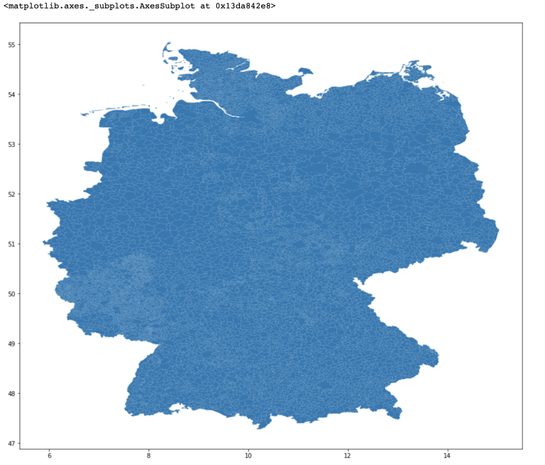
We will now do some visualisations working with GeoPandas and shapefiles. GeoPandas extends the datatypes used by pandas to allow spatial operations on geometric types. Shapefiles are geospatial vector data formats that allow for storing of geographic type features such as lines, points and polygons (areas). There are many shapefiles available on the internet. I am using one I found for Germany and have included this is the the github repo containing this notebook so you can replicate. Here we just read in the file (I have also printed it so you can take a look at it) and then plot it using matplotlib.
gdf = gpd.read_file('/Users/jasonram/Downloads/gadm36_DEU_shp/gadm36_DEU_4.shp')
print(gdf)
GID_0 NAME_0 GID_1 NAME_1 GID_2 \
0 DEU Germany DEU.1_1 Baden-Württemberg DEU.1.1_1
1 DEU Germany DEU.1_1 Baden-Württemberg DEU.1.1_1
2 DEU Germany DEU.1_1 Baden-Württemberg DEU.1.1_1
3 DEU Germany DEU.1_1 Baden-Württemberg DEU.1.1_1
4 DEU Germany DEU.1_1 Baden-Württemberg DEU.1.1_1
... ... ... ... ... ...
11297 DEU Germany DEU.16_1 Thüringen DEU.16.22_1
11298 DEU Germany DEU.16_1 Thüringen DEU.16.22_1
11299 DEU Germany DEU.16_1 Thüringen DEU.16.22_1
11300 DEU Germany DEU.16_1 Thüringen DEU.16.22_1
11301 DEU Germany DEU.16_1 Thüringen DEU.16.22_1
NAME_2 GID_3 NAME_3 GID_4 \
0 Alb-Donau-Kreis DEU.1.1.1_1 Allmendingen DEU.1.1.1.1_1
1 Alb-Donau-Kreis DEU.1.1.1_1 Allmendingen DEU.1.1.1.2_1
2 Alb-Donau-Kreis DEU.1.1.2_1 Blaubeuren DEU.1.1.2.1_1
3 Alb-Donau-Kreis DEU.1.1.2_1 Blaubeuren DEU.1.1.2.2_1
4 Alb-Donau-Kreis DEU.1.1.3_1 Blaustein DEU.1.1.3.1_1
... ... ... ... ...
11297 Weimarer Land DEU.16.22.9_1 Nordkreis Weimar DEU.16.22.9.12_1
11298 Weimarer Land DEU.16.22.9_1 Nordkreis Weimar DEU.16.22.9.13_1
11299 Weimarer Land DEU.16.22.9_1 Nordkreis Weimar DEU.16.22.9.14_1
11300 Weimarer Land DEU.16.22.9_1 Nordkreis Weimar DEU.16.22.9.15_1
11301 Weimarer Land DEU.16.22.9_1 Nordkreis Weimar DEU.16.22.9.16_1
NAME_4 VARNAME_4 TYPE_4 ENGTYPE_4 CC_4 \
0 Allmendingen None Gemeinde Town 084255001002
1 Altheim None Gemeinde Town 084255001004
2 Berghülen None Gemeinde Town 084255002017
3 Blaubeuren None Stadt Town 084255002020
4 Blaustein None Stadt Town 084250141141
... ... ... ... ... ...
11297 Rohrbach None Gemeinde Town 160715013081
11298 Sachsenhausen None Gemeinde Town 160715013082
11299 Schwerstedt None Gemeinde Town 160715013085
11300 Vippachedelhausen None Gemeinde Town 160715013092
11301 Wohlsborn None Gemeinde Town 160715013097
geometry
0 (POLYGON ((9.747226715087947 48.32448959350592...
1 (POLYGON ((9.76099872589117 48.32106399536138,...
2 POLYGON ((9.82752799987793 48.45702743530279, ...
3 POLYGON ((9.775817871093693 48.36040115356457,...
4 POLYGON ((9.82752799987793 48.45702743530279, ...
... ...
11297 POLYGON ((11.37983036041265 51.07011032104498,...
11298 POLYGON ((11.39456176757824 51.03350448608404,...
11299 POLYGON ((11.30850887298595 51.05867004394531,...
11300 POLYGON ((11.19609355926508 51.10009002685547,...
11301 POLYGON ((11.37327384948736 51.02006912231445,...
[11302 rows x 15 columns]
fig,ax = plt.subplots(figsize =(15,15))
gdf.plot(ax=ax)
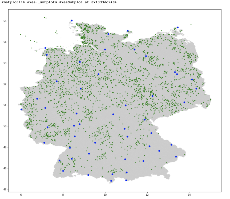
Next we just convert our df dataframe containing all our windfarm geometry points and our location dataframe that contains the location of our weather monitoring stations to GeoDataFrames and plot both the map, and overlay our windfarms as green dots and our weather monitoring stations as blue dots. Data basis: Deutscher Wetterdienst, gridded data reproduced graphically.
gdf2 = GeoDataFrame(df,geometry=geometry)
gdf2 = gdf2[(gdf2['Longitude'] >=5) & (gdf2['Longitude'] <20)]
gdf3 = GeoDataFrame(location,geometry=geometry2)
fig, ax = plt.subplots(figsize= (15,15))
gdf.plot(ax=ax,alpha = 0.4,color="grey")
gdf2.plot(ax=ax, color = "green", markersize = 5)
gdf3.plot(ax=ax, color = "blue", markersize = 30)
Get temperature data
Here we are using hourly air temperature. This could be a demand side feature as colder temperatures might lead to more heating use or warmer temperatures might lead to more airconditioning etc. Note we are only taking the data from one station in middle of Germany, but for our exploratory purposes this will give us some indication of temperature conditions. Data basis: Deutscher Wetterdienst. More information is available in the Further Resources section.
temp = pd.read_csv('/Users/jasonram/Downloads/DEairtemp.csv')
temp.set_index('Date', inplace=True)
temp.index = pd.to_datetime(temp.index)
temp.head()
| AirTemp | |
| Date | |
| 2016-01-14 00:00:00 | 2.9 |
|---|---|
| 2016-01-14 01:00:00 | 2.8 |
| 2016-01-14 02:00:00 | 2.6 |
| 2016-01-14 03:00:00 | 2.1 |
| 2016-01-14 04:00:00 | 1.6 |
wind = wind.join(temp, how='inner', on='Date')
wind.head()
| 10020 | 10046 | 10055 | 10091 | 10113 | 10147 | 10162 | 10200 | 10224 | 10264 | ... | 10908 | 10929 | 10946 | 10948 | 10961 | 10962 | TotWin | MeanTot | Output MwH | AirTemp | |
|---|---|---|---|---|---|---|---|---|---|---|---|---|---|---|---|---|---|---|---|---|---|
| Date | |||||||||||||||||||||
| 2016-01-14 00:00:00 | 5.1 | 3.1 | 4.1 | 4.1 | 5.1 | 4.1 | 4.1 | 4.1 | 5.1 | 3.1 | ... | NaN | 3.1 | 2.1 | 2.1 | 13.9 | 7.2 | 194.9 | 7.955102 | 9561.25 | 2.9 |
| 2016-01-14 01:00:00 | 4.1 | 3.1 | 3.1 | 5.1 | 4.1 | 5.1 | 4.1 | 5.1 | 5.1 | 3.1 | ... | NaN | 2.1 | 3.1 | 2.1 | 12.9 | 8.2 | 189.0 | 7.560000 | 9201.25 | 2.8 |
| 2016-01-14 02:00:00 | 5.1 | 3.1 | 3.1 | 4.1 | 4.1 | 5.1 | 4.1 | 3.1 | 4.1 | 3.1 | ... | NaN | 2.1 | 3.1 | 3.1 | 12.9 | 8.2 | 184.8 | 7.542857 | 8975.25 | 2.6 |
| 2016-01-14 03:00:00 | 5.1 | 3.1 | 3.1 | 5.1 | 4.1 | 5.1 | 3.1 | 5.1 | 4.1 | 3.1 | ... | NaN | 1.0 | 3.1 | 2.1 | 14.9 | 6.2 | 171.5 | 7.000000 | 8285.75 | 2.1 |
| 2016-01-14 04:00:00 | 1.0 | 3.1 | 5.1 | 3.1 | 4.1 | 4.1 | 4.1 | 4.1 | 3.1 | 3.1 | ... | NaN | 1.0 | 3.1 | 1.0 | 10.8 | 4.1 | 156.0 | 6.500000 | 8373.25 | 1.6 |
5 rows × 55 columns
Data on Solar energy
Here we are using hourly sum of solar incoming radiation data. At night the sun does not shine - so we should expect zero readings and from sunrise it should start to increase till sunset. Note, this is for only one area in the centre of Germany but for our exploratory purposes it will at least give us some indication on sunny conditions. Data basis: Deutscher Wetterdienst More information is available in the Further Resources section.
solar = pd.read_csv('/Users/jasonram/Downloads/DEsolar.csv')
solar.set_index('Date', inplace=True)
solar.index = pd.to_datetime(solar.index)
solar
| FG_LBERG | |
| Date | |
| 2016-01-14 00:00:00 | 0 |
|---|---|
| 2016-01-14 01:00:00 | 0 |
| 2016-01-14 02:00:00 | 0 |
| 2016-01-14 03:00:00 | 0 |
| 2016-01-14 04:00:00 | 0 |
| ... | ... |
| 2020-09-30 20:00:00 | 0 |
| 2020-09-30 21:00:00 | 0 |
| 2020-09-30 22:00:00 | 0 |
| 2020-09-30 23:00:00 | 0 |
| 2020-10-01 00:00:00 | 0 |
wind = wind.join(solar, how='inner', on='Date')
wind.head()
| 10020 | 10046 | 10055 | 10091 | 10113 | 10147 | 10162 | 10200 | 10224 | 10264 | ... | 10929 | 10946 | 10948 | 10961 | 10962 | TotWin | MeanTot | Output MwH | AirTemp | FG_LBERG | |
|---|---|---|---|---|---|---|---|---|---|---|---|---|---|---|---|---|---|---|---|---|---|
| Date | |||||||||||||||||||||
| 2016-01-14 00:00:00 | 5.1 | 3.1 | 4.1 | 4.1 | 5.1 | 4.1 | 4.1 | 4.1 | 5.1 | 3.1 | ... | 3.1 | 2.1 | 2.1 | 13.9 | 7.2 | 194.9 | 7.955102 | 9561.25 | 2.9 | 0 |
| 2016-01-14 01:00:00 | 4.1 | 3.1 | 3.1 | 5.1 | 4.1 | 5.1 | 4.1 | 5.1 | 5.1 | 3.1 | ... | 2.1 | 3.1 | 2.1 | 12.9 | 8.2 | 189.0 | 7.560000 | 9201.25 | 2.8 | 0 |
| 2016-01-14 02:00:00 | 5.1 | 3.1 | 3.1 | 4.1 | 4.1 | 5.1 | 4.1 | 3.1 | 4.1 | 3.1 | ... | 2.1 | 3.1 | 3.1 | 12.9 | 8.2 | 184.8 | 7.542857 | 8975.25 | 2.6 | 0 |
| 2016-01-14 03:00:00 | 5.1 | 3.1 | 3.1 | 5.1 | 4.1 | 5.1 | 3.1 | 5.1 | 4.1 | 3.1 | ... | 1.0 | 3.1 | 2.1 | 14.9 | 6.2 | 171.5 | 7.000000 | 8285.75 | 2.1 | 0 |
| 2016-01-14 04:00:00 | 1.0 | 3.1 | 5.1 | 3.1 | 4.1 | 4.1 | 4.1 | 4.1 | 3.1 | 3.1 | ... | 1.0 | 3.1 | 1.0 | 10.8 | 4.1 | 156.0 | 6.500000 | 8373.25 | 1.6 | 0 |
5 rows × 56 columns
Getting Prices Data (our Labels)
Thus far we have been building our feature matrix (our wind, temperature and solar features) and now we wish to build our label dataset - in our case we wish to look at hourly EPEX Spot energy prices. All price data on Refinitiv Platforms is in GMT - whereas all the ther data is in local (CET) - therefore we need to shift our price data forward by 1hr to align it correctly. The source is our Point Connect repository - again have included this file in the github repo so you can replicate.
pri = pd.read_csv('/Users/jasonram/Downloads/DEUprices1.csv')
pri.set_index('Date', inplace=True)
pri.index = pd.to_datetime(pri.index)
pri = pri.shift(+1, freq='H')
pri.head()
| Val | |
| Date | |
| 2015-01-01 01:00:00 | 18.29 |
|---|---|
| 2015-01-01 02:00:00 | 16.04 |
| 2015-01-01 03:00:00 | 14.60 |
| 2015-01-01 04:00:00 | 14.95 |
| 2015-01-01 05:00:00 | 14.50 |
Sometimes ML routines can work better with smoothed data so I have included a moving average, I don't use it here but include it for reference.
pri['val_mav'] = pri['Val'].rolling(window=5).mean()
pri.head()
| Val | val_mav | |
|---|---|---|
| Date | ||
| 2015-01-01 01:00:00 | 18.29 | NaN |
| 2015-01-01 02:00:00 | 16.04 | NaN |
| 2015-01-01 03:00:00 | 14.60 | NaN |
| 2015-01-01 04:00:00 | 14.95 | NaN |
| 2015-01-01 05:00:00 | 14.50 | 15.676 |
b = list(pri.columns[0:2].values)
for col in b:
col_zscore = col + '_zscore'
pri[col_zscore] = (pri[col] - pri[col].mean())/pri[col].std(ddof=0)
pri
| Val | val_mav | Val_zscore | val_mav_zscore | |
|---|---|---|---|---|
| Date | ||||
| 2015-01-01 01:00:00 | 18.29 | NaN | -1.038734 | NaN |
| 2015-01-01 02:00:00 | 16.04 | NaN | -1.175974 | NaN |
| 2015-01-01 03:00:00 | 14.60 | NaN | -1.263808 | NaN |
| 2015-01-01 04:00:00 | 14.95 | NaN | -1.242459 | NaN |
| 2015-01-01 05:00:00 | 14.50 | 15.676 | -1.269908 | -1.270077 |
| ... | ... | ... | ... | ... |
| 2019-09-30 21:00:00 | 44.58 | 53.148 | 0.564845 | 1.152580 |
| 2019-09-30 22:00:00 | 34.60 | 50.032 | -0.043892 | 0.951123 |
| 2019-09-30 23:00:00 | 33.09 | 43.776 | -0.135996 | 0.546657 |
| 2019-10-01 00:00:00 | 31.58 | 38.624 | -0.228100 | 0.213568 |
| 2019-01-10 01:00:00 | 30.04 | 34.778 | -0.322033 | -0.035086 |
41617 rows × 4 columns
We also need to normalize our feature matrix before handing it to our ML routine.
wind_zs = wind
b = list(wind_zs.columns.values)
for col in b:
col_zscore = col + '_zscore'
wind_zs[col_zscore] = (wind_zs[col] - wind_zs[col].mean())/wind_zs[col].std(ddof=0) #this handles nan vals
wind_zs
| 10020 | 10046 | 10055 | 10091 | 10113 | 10147 | 10162 | 10200 | 10224 | 10264 | ... | 10929_zscore | 10946_zscore | 10948_zscore | 10961_zscore | 10962_zscore | TotWin_zscore | MeanTot_zscore | Output MwH_zscore | AirTemp_zscore | FG_LBERG_zscore | |
|---|---|---|---|---|---|---|---|---|---|---|---|---|---|---|---|---|---|---|---|---|---|
| Date | |||||||||||||||||||||
| 2016-02-02 00:00:00 | 6.99 | 14.496 | -1.727986 | -1.346367 | 13.9 | 7.2 | 15.9 | 13.9 | 9.8 | 8.2 | ... | 1.091376 | 1.648526 | -0.093817 | 1.818084 | 0.718598 | 3.204296 | 3.374194 | 2.282638 | -0.188402 | -0.251216 |
| 2016-03-02 00:00:00 | 13.78 | 19.312 | -1.313825 | -1.035001 | 17.0 | 9.8 | 19.0 | 18.0 | 11.8 | 10.8 | ... | 1.091376 | 1.648526 | 0.710983 | 2.332151 | 2.516744 | 2.925399 | 3.074240 | 1.936871 | -0.939298 | -0.251216 |
| 2016-04-02 00:00:00 | 25.03 | 28.906 | -0.627622 | -0.414725 | 10.8 | 5.1 | 12.9 | 11.8 | 14.9 | 5.1 | ... | 0.445495 | 1.648526 | NaN | 0.764248 | 1.500401 | 1.385346 | 1.417906 | 0.989915 | -0.530722 | -0.251216 |
| 2016-05-02 00:00:00 | 26.62 | 30.968 | -0.530639 | -0.281412 | 7.2 | 3.1 | 7.2 | 7.2 | 4.1 | 2.1 | ... | 3.093606 | 1.648526 | 0.710983 | 1.021281 | 1.500401 | 0.348666 | 0.364528 | -0.381246 | -0.574892 | -0.251216 |
| 2016-06-02 00:00:00 | 26.41 | 32.474 | -0.543448 | -0.184045 | 9.8 | 4.1 | 5.1 | 8.7 | NaN | 6.2 | ... | -0.200385 | -0.111577 | -0.093817 | 0.481511 | -0.493195 | 0.178608 | 0.120055 | 0.277080 | 0.772304 | -0.251216 |
| ... | ... | ... | ... | ... | ... | ... | ... | ... | ... | ... | ... | ... | ... | ... | ... | ... | ... | ... | ... | ... | ... |
| 2019-09-30 20:00:00 | 49.27 | 52.510 | 0.850916 | 1.111332 | 8.2 | 4.1 | 10.8 | 12.9 | 6.2 | 3.1 | ... | -0.200385 | -1.079634 | -0.979097 | -0.161072 | -0.102294 | 0.287445 | 0.179243 | 0.689498 | 0.032450 | -0.251216 |
| 2019-09-30 21:00:00 | 44.58 | 53.148 | 0.564845 | 1.152580 | 7.2 | 4.1 | 10.8 | 12.9 | 3.1 | 5.1 | ... | -0.200385 | -0.111577 | -0.979097 | 0.352995 | -0.884097 | 0.179968 | 0.121518 | 0.518119 | 0.087663 | -0.251216 |
| 2019-09-30 22:00:00 | 34.60 | 50.032 | -0.043892 | 0.951123 | 7.2 | 3.1 | 9.8 | 12.9 | 3.1 | 4.1 | ... | -0.910854 | -1.079634 | -0.979097 | 0.764248 | -0.884097 | 0.034398 | -0.087575 | 0.468959 | 0.142876 | -0.251216 |
| 2019-09-30 23:00:00 | 33.09 | 43.776 | -0.135996 | 0.546657 | 6.2 | 3.1 | 8.7 | 10.8 | 6.2 | 4.1 | ... | -0.200385 | -1.079634 | -0.979097 | 1.818084 | -1.314088 | 0.141875 | 0.025751 | 0.379867 | 0.164961 | -0.251216 |
| 2019-10-01 00:00:00 | 31.58 | 38.624 | -0.228100 | 0.213568 | 7.2 | 4.1 | 6.2 | 7.2 | 8.7 | 3.1 | ... | -0.200385 | -1.079634 | NaN | -0.700842 | -0.102294 | 0.345945 | 0.361541 | 0.635634 | 0.054536 | -0.251216 |
30977 rows × 116 columns
Temporal Considerations
We want to compare the same hourly data for each day - so we need to create a daily series for each hour in the day as it is these series we want to model. The reason is that demand/supply profiles are different each hour of the day so - its not correct to compare hours in a continuous series ie hour 01 to hour 02 etc. The correct set up should be day 1 hour 1, day 2 hour 1, day 3 hour 1 etc. In this way we build up 24 discrete hourly profiles - as it is these we wish to model. Below we just extract the hour of our timestamp.
intersected_df['hour'] = intersected_df.index.strftime('%H')
Implement Machine Learning Model
For our modelling we will use an xgboost model - which a gradient-boosted decision tree class of algorithm - which is quite popular in the literature. We will apply the simplest vanilla implementation here to see if we can get any usable results. Obviously the ML area is quite technical and requires some mastery but you can use this codebase to extend and experiement as appropriate.
Split our dataset in to train, evaluation and test sets
We need to split our dataset into a training set, an evaluation set and a test set. We will hand the the ML routine only the training and evaluation datasets to generate its models. We will then test predictions made by that model against the test dataset to see if we can find anything useful. We split the data roughly at the halfway mark using 10% of our data as evaluation set.
hour_ls = intersected_df.hour.unique()
hour_ls
array(['00', '01', '02', '03', '04', '05', '06', '07', '08', '09', '10',
'11', '12', '13', '14', '15', '16', '17', '18', '19', '20', '21',
'22', '23'], dtype=object)
split_date = '2017-10-01'
eval_date = '2017-12-01'
pri_train = {}
pri_eval = {}
pri_test = {}
for h in hour_ls:
pri_train[h] = pd.DataFrame((intersected_df.loc[(intersected_df.index <= split_date)
& (intersected_df['hour']== h)].copy()),
columns = intersected_df.columns)
pri_eval[h] = pd.DataFrame((intersected_df.loc[(intersected_df.index > split_date)
& (intersected_df.index <= eval_date)
& (intersected_df['hour']== h)].copy()),
columns = intersected_df.columns)
pri_test[h] = pd.DataFrame((intersected_df.loc[(intersected_df.index > eval_date)
& (intersected_df['hour']== h)].copy()),
columns = intersected_df.columns)
for h in hour_ls:
print(h,pri_train[h].shape, pri_eval[h].shape, pri_test[h].shape)
00 (606, 117) (60, 117) (609, 117)
01 (611, 117) (61, 117) (634, 117)
02 (610, 117) (61, 117) (637, 117)
03 (602, 117) (61, 117) (624, 117)
04 (611, 117) (61, 117) (626, 117)
05 (610, 117) (61, 117) (628, 117)
06 (594, 117) (58, 117) (572, 117)
07 (611, 117) (60, 117) (632, 117)
08 (610, 117) (61, 117) (633, 117)
09 (598, 117) (61, 117) (589, 117)
10 (612, 117) (61, 117) (635, 117)
11 (613, 117) (61, 117) (631, 117)
12 (591, 117) (60, 117) (612, 117)
13 (613, 117) (61, 117) (634, 117)
14 (613, 117) (61, 117) (637, 117)
15 (598, 117) (60, 117) (614, 117)
16 (609, 117) (61, 117) (629, 117)
17 (608, 117) (61, 117) (630, 117)
18 (588, 117) (59, 117) (610, 117)
19 (607, 117) (61, 117) (631, 117)
20 (611, 117) (61, 117) (637, 117)
21 (599, 117) (61, 117) (619, 117)
22 (612, 117) (61, 117) (637, 117)
23 (612, 117) (61, 117) (633, 117)
Create feature and label sets
We now need to seperate our training (pri_train), evaluation (pri_eval) and test (pri_test) dataframes into their feature and label set components. Here we create a small function to do this for us. The training, evaluation and test datasets contain both the raw and the normalised (_zscore) data. We only wish to pass the normalised feature data to the ML routine so we simply select the relevant zscore features. The function also takes in which target label parameter, which we use to select the column we want to model for.
def create_features(df, label=None):
collist = df.columns.tolist()
relcols = collist[60:len(collist)-1]
X = df[relcols]
if label:
y = df[label].to_frame()
return X, y
return X
Define our XGBoost model - hand it our train, eval and test sets
So we are now ready to hand each of our 3 datasets for each hour from 0 to 23 to the XGBoost routine to generate a model for each hour. We define our XGB model using the Regressor class and a squared error objective function. We then pass the training feature and label sets to the fit function along with our evalution set. Once the modeel is generated, we will then store the feature importance graph and then generate a prediction for each hour and then calculate the Mean Squared Error (MSE) for each prediction versus the observed label.
ax_ls ={}
res ={}
reg = xgb.XGBRegressor(objective ='reg:squarederror',n_estimators=1000)
for h in hour_ls:
#create our features, train, eval & test
X_train, y_train = create_features(pri_train[h], label='Val_zscore')
X_eval, y_eval = create_features(pri_eval[h], label='Val_zscore')
X_test, y_test = create_features(pri_test[h], label='Val_zscore')
#define our xgboost model
reg.fit(X_train, y_train,
eval_set=[(X_eval, y_eval)],
early_stopping_rounds=50,
verbose=False)
#create and store feature importance plots
ax_ls[h]= reg.get_booster().get_fscore()
#create prediction from our xgboost model
pri_test[h]['ML_Prediction'] = reg.predict(X_test)
#calculate prediction accuracy using MSE
res[h] = mean_squared_error(pri_test[h]['Val_zscore'].values, pri_test[h]['ML_Prediction'].values)
Generate Visual Output
We have just created 24 hourly xgboost models, we now want to plot our feature importance (the higher the F-score the more important the feature) for each hourly series, as well as the accuracy of our ML generated predictions - using in our case the mean squared error (MSE) calculation we created above. We can easily do this is 2 steps.
fig = plt.figure(figsize=(20,60))
for i,col in enumerate(hour_ls):
bx=plt.subplot(15,2,i+1)
data1 = OrderedDict(sorted(ax_ls[col].items(), key=lambda t: t[1]))
plt.barh(range(len(data1)),data1.values(), align='center')
plt.yticks(range(len(data1)),list(data1.keys()))
plt.title = ("Hour " + col)
plt.show()
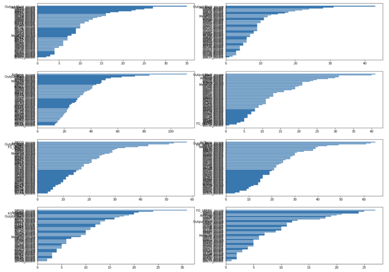
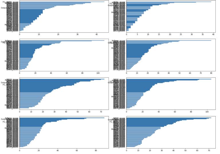
fig = plt.figure(figsize=(20,60))
for i,col in enumerate(hour_ls):
ax=plt.subplot(15,2,i+1)
pri_test[col][['Val_zscore','ML_Prediction']].plot(ax=ax,legend=False,title = ("Hour " + col) )
props = dict(boxstyle='round', facecolor='wheat', alpha=0.5)
ax.set_xlabel('xlabel', fontsize=6)
ax.set_ylabel('ylabel', fontsize=3)
ax.text(0.75, .15, "MSE: " + str(round(res[col],2)), transform=ax.transAxes, fontsize=13,
verticalalignment='bottom',bbox=props)
plt.xticks(rotation=90)
plt.show()
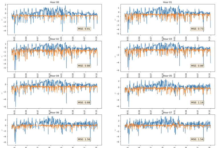
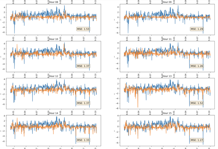
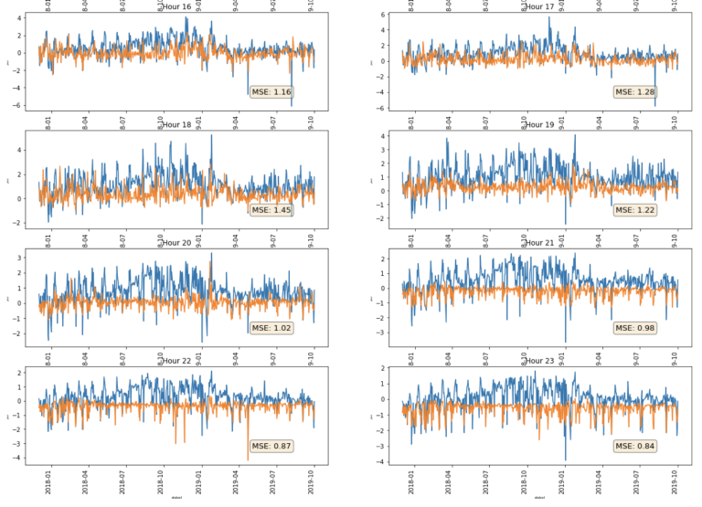
Initial Observations
From the line charts above, we can see that the generated models are able to predict some of the downward spikes in spot energy prices. The MSE varies from 0.73 (hour 01) to 1.56 (hour 6). There does seem to be quite some variation in accuracy even with this very simple and limited model. However, none of these are particularly accurate, MSE of 0 being perfect and MSE of 1 indicating 1 standard deviation.
We can see for example that on some days prices went much lower than our prediction - this could be due for example to a day which was both windy and sunny (remember these energy sources are not stored but dumped to the grid - leading to the negative prices - the negative prices discourage use of thermal sources). We did have one feature included for solar energy - but it was for only one location in the centre of the country, as opposed to wind which we had much greater coverage for. Conversely, there are other days where the prediction was much lower than the observed, so perhaps it wasn't that sunny at all locations or thermal capacity had been dialled back etc. So we could expand our model to include new more complete features such more solar locations, thermal features and such.
Our model does not really tell us anything about upward spikes as we have only included one demand side type of feature - air temperature - and only for one station in the centre of Germany - in our feature matrix. Again we could expand our model with features that might help us with this demand side modelling for example.
Another next step might be to use only a subset of the highest F-score features and re-run the models to see if that can improve things, or indeed look at a suite of different classes of algorithm - we have only used xgboost but there are many other that we could implement within the main iterative routine I have given above.
Further, we have been looking only at observed values. Remember, one of the features we are using is actual Wind Output - we wouldn't know this ahead of time. So clearly we need to know about forecast data. We know that energy markets are based around forecast data. So another next step would be to incorporate all of that data but that is beyond the scope of this introductory article.
Summary
A lot of ground was covered in this article so let's summarize. We retrieved a set of physical asset (windfarms in our case) RICs from our excellent new RDP Search API. We used these to request some reference-type data for these windfarms using our Eikon Data API. We then created a new geometry 'Point' datatype where we stored locational co-ordinates for our windfarms. We followed this by loading some open source wind data, wind output data from our Point Connect repository and joined these together, creating 2 additional features along the way. We also loaded some open source solar energy and air temperature data. We then retrived the locations of our weather monitoring stations and as before, created a new geometry datatype for those. We were then able to calculate the closest weather monitoring station for each of our windfarms using the scipy.spatial cdist routine - though we didn't use it in ths introductory model other than for visualisation - I included it as it might prove useful were you to develop more complex models. We then downloaded a shape file for Germany, converted our pandas dataframes to GeoPandas dataframes and ploted overlays for both windfarms and wind monitoring stations. Next we read in some price data (EPEX Spot) to use for our label data, shifted it forward one hour to align with our local time (CET) features and we then started to normalise our datasets using z-scores. After joining our feature and label dataframes, we then added a feature called hour which tells us which hour the timestamp refers to. We then split our data into training, evaluation and test sets and defined our feature and label sets for each of the 24 hours in the day. Next we defined 24 different XGBoost ML models (one for each hour of the day), handing it the appropriate training and evaluation sets and ploted our feature importance F-scores. Finally, we used our model to generate a label prediction based on our hold-out or test feature matrix and plotted that against the observed label values.
Whilst a simple and far from complete example, I hope this article can provide you with an idea of how to approach this area and a practical codebase to experiment and explore further.
Further Resources
Further Resources for Eikon Data API
For Content Navigation in Eikon - please use the Data Item Browser Application: Type 'DIB' into Eikon Search Bar.
Further Resources for Refinitv Data Plaform (RDP) APIs
For Content Navigation in RDP - please go here
For more information on the Point Connect service please go here
Further Resources for Open Source German Weather Data kindly made public by DWD
Hourly Air Temperature - I used Station 01266, and field TT_TU
Hourly Solar Readings - I used Station 00183, and field FG_LBERG
Source of geospatial base data:
Surveying authorities of the Länder and Federal Agency for Cartography and Geodesy (https://www.bkg.bund.de).
Source of satellite data: EUMETSAT (https://www.eumetsat.int) NOAA (https://www.noaa.gov)
Further Resources for Shapefiles