/rdp2.jpeg)

UPDATE as of JAN 2022:
Statement from the RDP Library team:
Refinitiv Data Platform Libraries (RDP libraries) have been redesigned and renamed to Refinitiv Data Libraries (RD libraries). Alpha versions of former RDP libraries will be maintained for a while, but for new development, it is recommended to use the latest RD libraries which incorporate new features and offer greater usability. Please refer to the following pages for more about the new RD libraries: RD library for Python, RD Library for TypeScript (Q1 2022), RD Library for .NET.
Original article:
As part of our 2019 Refinitiv Developer Days Series, I spent a few months travelling around Europe giving members of our developer community a sneak peek at our exciting new Refinitiv Data Platform Library.
The feedback was so positive, I felt it was only right to share this with our wider community - showcasing some of the key features which will make the Refinitiv Data Platform Library such a useful addition to our current set of APIs.
This is Part 2 of this exploration of the new Library, so if you have not already done so - I recommend you check out Part 1 first.
As mentioned in part 1 of this article, the Refinitiv Data Platform Library is in Alpha mode and was released as part of an Early Access Programme in the first weeks of January 2020.
The latest alpha version of the Python library can be obtained on PyPi - install by executing 'pip install refinitiv-dataplatform' - in your Python environment.
Likewise, the .NET version can be found on NuGet - the base package and the Content Layer - with installation instructions on the relevant pages.
You can also find sample code on GitHub in .NET and Python flavours.
One Library - Three Abstraction Layers
Just to recap, to cater to all developer types, the library offers 3 abstraction layers from the easiest to the slightly(!) more complex.
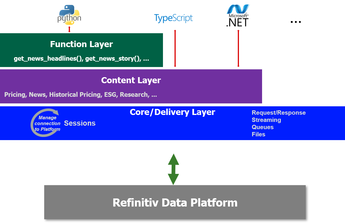
The three layers are as follows:
- Function: Highest level - single function call to get data
- Content: High level - Fuller response and Level 1 Streaming data too
- Delivery: For Level 2 Streaming data and data sets not supported by above Layers
We have already explored the Function and Content Layer in Part 1 of this article so let us now move onto the Delivery Layer
Delivery Layer
As I mentioned in Part 1, Refinitiv will continue to develop the library and hope to offer Function and Content layer support for other content types such as ESG data, Symbology, Streaming Chains, Bonds and so on.
However, if you want to access Data which is not currently supported by the other Layers - or which most likely won't be supported - such as Level 2 Streaming Data - then you will need to use the Delivery layer.
The Delivery is slightly more complex than the Content Layer - but as I will hopefully demonstrate, not onerously so.
In this 2nd part of the sneak peek, I will highlight the access of content such as Realtime Streaming Level 2 data, ESG Data, Surfaces and Curves with relative ease using the Delivery Layer.
Streaming Level 2 Data
In Part 1 of this article, we looked at using the Content Layer to consume Streaming Market Price data - which is often referred to as Level 1 data - things like Trade and Quote data representing basic Market activity.
Using the Delivery layer we can also consume Level 2 data - including Full Depth Market Order Books.
One example of Full Depth Order Book available from Refinitiv is Market By Price data - also known as a Market Depth Aggregated Order Book - consisting of a 'collection of orders for an instrument grouped by Price point i.e. multiple orders per ‘row’ of data'.
Streaming MarketByPrice request
Let's go ahead and request some MarketByPrice data for Vodafone on the LSE using the Delivery layer.
Assuming we have already established a session to the platform of our choice (see part 1), we can just go ahead and execute something like the following in Python:
order_book = rdp.OMMItemStream(session = session,
name = "VOD.L",
domain = "MarketByPrice",
on_refresh = lambda s, msg : print(json.dumps(msg, indent=2)),
on_update = lambda s, msg : print(json.dumps(msg, indent=2)),
on_status = lambda s, msg : print(json.dumps(msg, indent=2)))
order_book.open()
OR the something like in this C#
JObject image = new JObject();
using (IStream orderBook = DeliveryFactory.CreateStream(
new ItemStream.Params().Session(session)
.Name("VOD.L")
.WithDomain("MarketByPrice")
.OnRefresh((s, msg) => image.Merge(msg))
.OnComplete(s => DumpImage(image))
.OnUpdate((s, msg) => DumpUpdate(msg))
.OnStatus((s, msg) => Console.WriteLine(msg))))
{
// Open the stream...
orderBook.Open();
}
For both snippets, we pass in our Session, the Instrument name, some lambda functions, the Domain for the required type of data and finally open the Order Book stream.
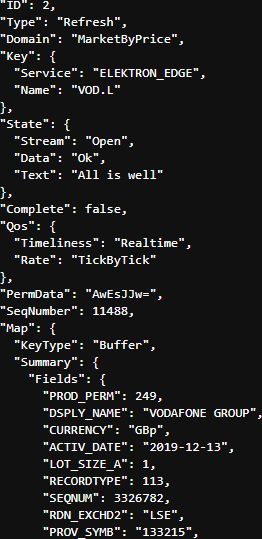
Assuming the request is valid, we should get back an Initial Refresh Msg representing the current state of the market for that instrument i.e. all open orders aggregated by price point.
At the start of the Refresh Msg you will see some header information including Summary Data - which contains non-order specific values like the Instrument name, the currency, most recent activity time, trading status, exchange ID and so on:
Following the Summary Data, you will receive the Order Book entries themselves:
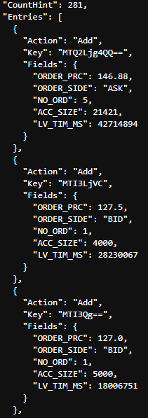
Here I have just pasted the first 3 of the 281 entries aggregated price points.
Once the complete Order Book has been delivered we can then expect to start receiving Update Msgs as the Market changes:
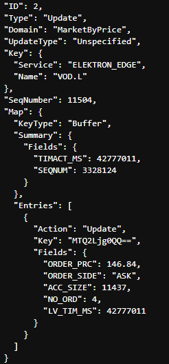
This Update Msg contains instructions to Update an existing Price Point in the Order Book.
Update Msgs can also contain instructions to Add new Price points and/or Delete existing Price Points to/from the Order Book.
In addition to MarketByPrice data, the Delivery Layers will allow the consuming other Level 2 Streaming Domains - including any Custom Domain models published on your internal Refinitiv Real-Time Distribution System (formerly known as TREP).
Non-Streaming Data from the Refinitiv Data Platform
As well as Streaming Data, the Delivery layer will also allow you to access data normally delivered using the Request-Response mechanism such as Historical, Symbology, Fundamentals, Analytics, research, ESG data and so on.
Endpoint Interface
In the 1st part of this article, I mentioned that Refinitiv is gradually moving much of their vast breadth and depth of content onto the Refinitiv Data Platform.
Each unique content set will have its own Endpoint on the Refinitiv Data Platform - to access that content, you can do so use using the Endpoint interface provided as part of the Delivery Layer.
ESG (Environmental, Social and Governance) data
One example of content not yet supported by the Function and Content Layer is ESG data. However, it can be accessed relatively easily as follows:
- Identify the Endpoint for ESG data
- Use the Endpoint Interface to send a request to the Endpoint
- Decode the response and extract the ESG data
Sounds simple enough, how does that work in practice?
Identifying the Endpoint
To ascertain the Endpoint, we can use the Refinitiv Data Platform's API Playground - which an interactive documentation site you can access once you have a valid Refinitiv Data Platform account.
So, firstly we search for 'env' to narrow down the list of Endpoints and then select the subset of the ESG data that we are interested in, for example - ESG Scores with full history:
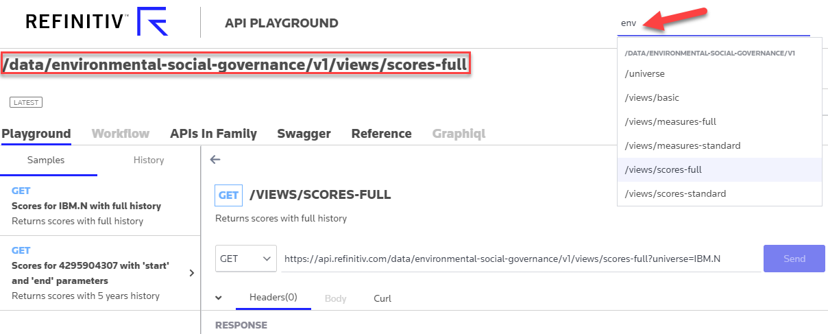
We then note the Endpoint URL - /data/environmental-social-governance/v1/views/scores-full - which can be used with the Endpoint interface as follows:
# python
endpoint_url = "data/environmental-social-governance/v1/views/scores-full"
endpoint = rdp.Endpoint(session, endpoint_url)
response = endpoint.send_request( query_parameters = {"universe": "IBM.N"} )
OR
// C#
var endpointUrl = "https://data/environmental-social-governance/v1/views/scores-full";
IEndpointResponse response = Endpoint.SendRequest(session, endpointUrl,
new Endpoint.Request.Params().WithQueryParameter("universe", "IBM.N"));
We create the Endpoint object, passing in our session and the URL and then use the Endpoint to request the data for whatever entity we want - for example IBM
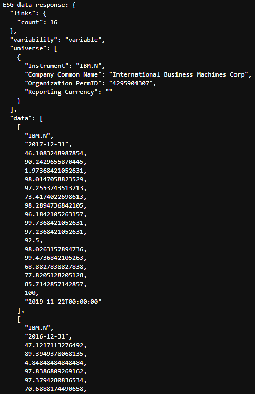
The payload is in JSON format and starts with some header information such as the number of years of scores (16) and some brief information on the organisation. After which we see the scores for each year, starting with the most recent.
You will, off course, find full documentation for each of the individual scores on the API playground - however, the JSON payload is self-describing and includes fairly verbose descriptions for the various scores at the end of the payload:
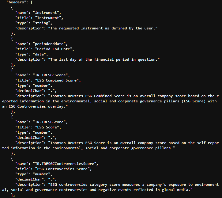
This saves us from having to cut and paste score names, descriptions etc from the documentation - instead we can just extract from the payload itself - particularly useful for GUI applications, displaying tooltips etc.
As the data is in JSON format, if we are working in Python, we can easily convert it to a Pandas DataFrame:
titles = [i["title"] for i in response.data.raw['headers']]
pd.DataFrame(response.data.raw['data'],columns=titles)
Will result in something like:
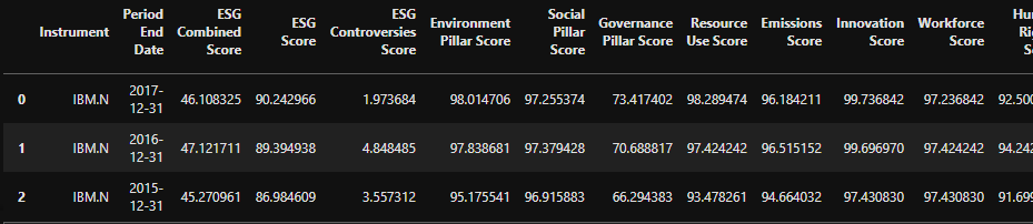
As you can see, even with the lowest level Delivery layer, it is still relatively straightforward to request advanced datasets and handle the response.
To illustrate this further, I would like to share a couple of other Endpoints that were demonstrated by one of my colleague's - Samuel Schwalm (Director, Enterprise Pricing Analytics) - at our recent London Developer Day event. I have picked these two Endpoints because I was amazed at just how easily you could access and display such rich data content. I expect that whilst you could do something similar in Excel, it would require much more effort and most likely involve several sheets of data, filters and Analytics functions.
Instrument Pricing Analytics - Volatility Surfaces Endpoint
The first example that Samuel showed us, used the Volatility Surfaces Endpoint.
Using the API Playground we can identify the Endpoint URL and create the Endpoint object:
endpoint = rdp.Endpoint(session,
"https://api.refinitiv.com/data/quantitative-analytics-curves-and-surfaces/v1/surfaces")
Then, using the reference documentation, we can build up our Request;
Suppose we want to compare volatility for Renault, Peugeot, BMW and VW - we can generate a volatility surface:
- from the Option Settle prices using an SSVI model
- express the axes in Dates and Moneyness
- and return the data in a matrix format
using the following request:
request_body={
"universe": [
{ "surfaceTag": "RENAULT",
"underlyingType": "Eti",
"underlyingDefinition": {
"instrumentCode": "RENA.PA"
},
"surfaceParameters": {
"inputVolatilityType": "settle",
"volatilityModel": "SSVI",
"xAxis": "Date",
"yAxis": "Moneyness"
},
"surfaceLayout": { "format": "Matrix", }
},
{ "surfaceTag": "PEUGEOT",
"underlyingType": "Eti",
"underlyingDefinition": {
"instrumentCode": "PEUP.PA"
},
"surfaceParameters": {
"inputVolatilityType": "settle",
"volatilityModel": "SSVI",
"xAxis": "Date",
"yAxis": "Moneyness"
},
"surfaceLayout": {"format": "Matrix" }
},
{ "surfaceTag": "BMW",
"underlyingType": "Eti",
"underlyingDefinition": {
"instrumentCode": "BMWG.DE"
},
"surfaceParameters": {
"inputVolatilityType": "settle",
"volatilityModel": "SSVI",
"xAxis": "Date",
"yAxis": "Moneyness"
},
"surfaceLayout": {"format": "Matrix" }
},
{ "surfaceTag": "VW",
"underlyingType": "Eti",
"underlyingDefinition": {
"instrumentCode": "VOWG.DE"
},
"surfaceParameters": {
"inputVolatilityType": "settle",
"volatilityModel": "SSVI",
"xAxis": "Date",
"yAxis": "Moneyness"
},
"surfaceLayout": {"format": "Matrix" }
}],
"outputs":["forwardCurve", "dividends"]
}
And then we send the request to the Platform:
response = endpoint.send_request(
method = rdp.Endpoint.RequestMethod.POST,
body_parameters = request_body
)
Once we get the response back, we can extract the payload and use the Matplotlib to library to plot our data.
surfaces = response.data.raw['data']
plot_surface(surfaces, 'VW')
Where the code for our plot_surfaces helper is as follows:
def plot_surface(surfaces, surfaceTag):
#various imports removed for brevity
surfaces = pd.DataFrame(data=surfaces)
surfaces.set_index('surfaceTag', inplace=True)
surface = surfaces[surfaces.index == surfaceTag]['surface'][0]
strike_axis = surface[0][1:]
surface = surface[1:]
time_axis = []
surface_grid = []
for line in surface:
time_axis.append(line[0])
surface_grid_line = line[1:]
surface_grid.append(surface_grid_line)
time_axis = convert_yyyymmdd_to_float(time_axis)
x = np.array(strike_axis, dtype=float)
y = np.array(time_axis, dtype=float)
ero = np.array(surface_grid, dtype=float)
X,Y = np.meshgrid(x,y)
fig = plt.figure(figsize=[15,10])
ax = plt.axes(projection='3d')
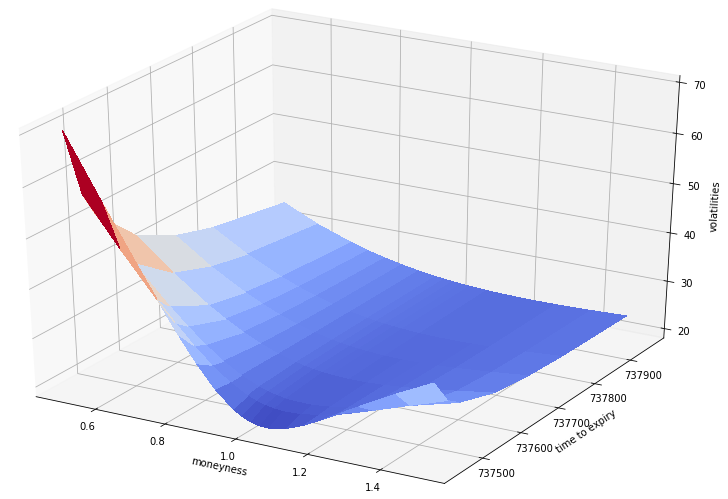
ax.set_xlabel('moneyness')
ax.set_ylabel('time to expiry')
ax.set_zlabel('volatilities')
surf = ax.plot_surface(X,Y,Z, cmap=cm.coolwarm, linewidth=0, antialiased=False)
plt.show()
Python code to display the volatility surface of the specified company
Resulting in our lovely Surface plot:
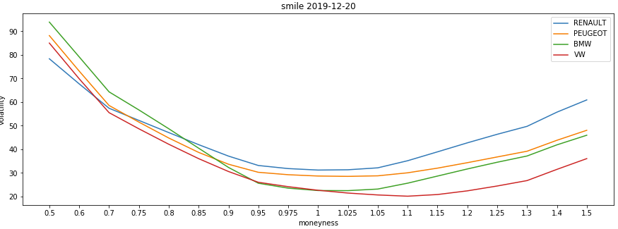
Smile Curve
We can also use the same surfaces response data to plot a Smile Curve.
For example, to compare the volatility smiles of the 4 equities at the chosen time expiry (where the maturity value of 1 is the first expiry):
plot_smile(surfaces, 1)
def plot_smile(surfaces, maturity):
#various imports removed for brevity
fig = plt.figure(figsize=[15,5])
ax = plt.axes()
ax.set_xlabel('moneyness')
ax.set_ylabel('volatility')
surfaces = pd.DataFrame(data=surfaces)
for i in range(0,surfaces.shape[0]):
label = surfaces.loc[i,['surfaceTag']]['surfaceTag']
surface = surfaces.loc[i,['error','surface']]['surface']
error = surfaces.loc[i,['error']]['error'] if 'error' in surfaces else 0.0
#print ("error = surfaces.loc[i,['error']]['error'] if 'error' in surfaces else 0")
x=[]
y=[]
if (type(error) is float):
x = surface[0][1:]
y = surface[maturity][1:]
title = 'smile ' + str(surface[maturity][0])
ax.set_title(title)
ax.plot(x,y,label=label)
plt.legend()
plt.show()
Produces something like this:
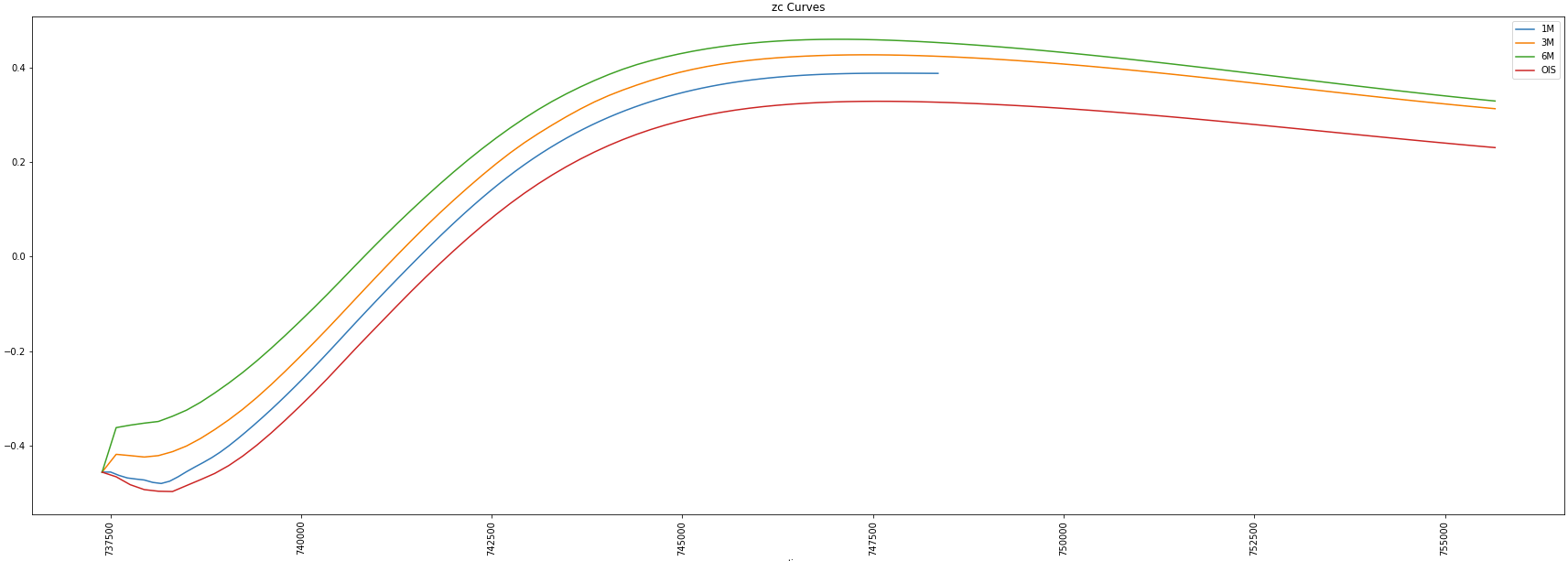
Instrument Pricing Analytics - Zero-Coupon Curves Endpoint
Another example that Samuel showed us during the London Developer day, used the Zero-Coupon Endpoint.
Using the API Playground documentation, we again determine the Endpoint URL, create the Endpoint object, build our request and send it to the Platform.
If we wanted to ask for:
- the swap-derived zero curves for the available EURIBOR tenors (1M, 3M, 6M)
- zc curves to be generated using an OIS discounting methodology
- mid swap market quotes to be used
- interpolation using cubic spline
- and any extrapolation to be done in a linear way
We would send the following request:
endpoint = rdp.Endpoint(session,
"https://api.refinitiv.com/data/quantitative-analytics-curves-and-surfaces/v1/curves/zcCurves")
request_body={
"universe": [
{
"curveParameters": {
"interpolationMode": "CubicSpline",
"priceSide": "Mid",
"interestCalculationMethod": "Dcb_Actual_Actual",
"extrapolationMode": "Linear"
},
"curveDefinition": {
"currency": "EUR",
"indexName": "EURIBOR",
"source": "Refinitiv",
"discountingTenor": "OIS",
}
}],
"outputs": ["Curves"]
}
response = endpoint.send_request(
method = rdp.Endpoint.RequestMethod.POST,
body_parameters = request_body
)
We can then use the payload response to display the curves generated for the 1M, 3M and 6M Eurobor swap as well as the EONIA cz curve used for discounting:
curves = response.data.raw['data'][0]
plot_zc_curves(curves, ['1M','3M','6M','OIS'])
def plot_zc_curves(curves, curve_tenors=None, smoothingfactor=None):
#imports removed for brevity
tenors = curve_tenors if curve_tenors!=None
else curves['description']['curveDefinition']['availableTenors'][:-1]
s = smoothingfactor if smoothingfactor != None else 0.0
fig = plt.figure(figsize=[30,10])
ax = plt.axes()
ax.set_xlabel('time')
ax.set_ylabel('zc rate')
title = 'zc Curves'
ax.set_title(title)
for tenor in tenors:
curve = pd.DataFrame(data=curves['curves'][tenor]['curvePoints'])
x = convert_ISODate_to_float(curve['endDate'])
y = curve['ratePercent']
xnew, ynew = smooth_line(x,y,100,s)
ax.plot(xnew,ynew,label=tenor)
plt.xticks(rotation='vertical')
plt.legend()
plt.show()
Which should produce something that looks like this:
Based on the above examples, I hope you will agree, that the Analytics Endpoints are incredibly versatile and powerful allowing you to perform complex analysis on the Platform using the latest market contributions in a straightforward yet flexible manner.
Additional Endpoints
At the time of writing, there are several other Endpoints - beta or released - currently defined on the Refinitiv Data Platform including, but not limited to:
- Alerts subscriptions for Research data, News and Headlines
- Company Fundamentals - such a Balance sheet, Cash flow, financial summary etc
- Symbology - symbol lookup to and from different symbology types
- Ultimate Beneficial Ownership
- Search - simple and structured
- Aggregates - e.g. Business Classifications
and with more to come as we onboard more of our content onto the Refinitiv Data Platform
Access to the Library EAP and the Platform itself
As mentioned earlier, an Alpha version of this Library was released as part of an Early Access Programme in the first weeks of January 2020 (see download links below).
If these two articles piqued your interest and you want to explore the Platform content for yourself, reach out to your Refinitiv representative to arrange a trial Platform account. The trial Platform account will give you access to the API Playground as well.
If you have any questions / suggestions or issues related to the library, please feel free to post on the Refinitiv Data Platform Library section of our Q&A Forum.
Additional Resources
You will find links to the Source code, APIs, Documentation and Related Articles in the Links Panel