
This article was written by the winner of 2021 Q.2 Refinitiv Academic Competition. It is aimed at Academics from Undergraduate level up.
Refinitiv Academic Article Competition
Refinitiv is pleased to host its Academic Article Competition.
This competition aims at helping students - from undergraduate to postdoctorate level - to publish their work on internationally recognized platforms and to aid them in (i) academic style writing, (ii) implementing code in their study, (iii) coding, (iv) financial knowledge, (v) developing a contacts network in the finance, and (vi) generating ideas for economics/finance papers.
It will have to be an economic or financial study, and in a style akin to these articles:
- Estimating Monthly GDP Figures Via an Income Approach and the Holt-Winters Model
- Beneish's M-Score and Altman's Z-Score for analyzing stock returns of the companies listed in the S&P500
- Information Demand and Stock Return Predictability (Coded in R)
- Computing Risk-Free Rates and Excess Returns from Zero-Coupon-Bonds
As per these examples, the length of the study in question is not a limit; there is no min. or max. length your article has to be to qualify. However, it needs to show and explain the code used in its study. It can be in any (reasonable) format (such as LaTeX, PDF, Word, Markdown, …) but it would preferably be a Jupyter Notebook (you may choose to use Refinitiv’s CodeBook to write it). You will also need to use Refintiv APIs/data-sets before being published on our Developer Portal – were it to win the competition.
There is no min. or max. number of winners; any work exceeding our standards will be selected for publication. Thus, do not hesitate to share this with your colleagues, informing them of this opportunity, they are not competitors, but collaborators; you may even choose to work together on this project.
We are ready and happy to provide any help in writing such articles. You can simply email Jonathan Legrand - the Competition Leader - at jonathan.legrand@refinitiv.com .
Abstract
This paper studies the implementation of deep learning to predict probability distributions. These describe the daily returns of stocks of the companies in the financial sector, listed in the S&P500, using the data obtained from the Refinitiv Eikon API from 2002 to 2020. In addition, it proposes an approach to obtain a relative probabilistic value defined as the predicted mean divided by the predicted standard deviation of the returns of a stock.
Using six variables, obtained from the financial statements of the companies, as input to predict the parameters of four chosen distributions (normal, JohnsonSU, a mixture of three normal distributions, a mixture of two Johnson distributions), the results obtained range from 7 to 518 BPS each year in the test set.
The proposed neural networks obtain lower losses in the test data (including the period of the Covid-19 of 2020) than in the training data, even when they have more than 1400 trainable parameters without regularization nor dropout layers. Although it requires further study, the prediction of a probability distribution of returns allows for more informed decisions, showing an alternative use of deep learning for predicting stock returns.
1. Introduction
Multiple methods have been developed to estimate the fair value of a company under varying assumptions. Nevertheless, most of these methods produce a single value estimate, which might not be enough for an investor to make a wise investment decision. A valuation model returning not only the expected value of the stock but also the risks of this estimate is proposed as a better approach to make economic decisions.
In that sense, this paper aims to develop a valuation method that estimates a distribution of future returns for each stock. Making it valid for comparison not only for mean results but also for the probabilities of different returns. The five elements in which the return on equity can be decomposed through the DuPont analysis and the dividend payout rate are used as inputs to a neural network model, which produces the parameters of the distribution. These predicted distributions of returns are then used for comparing stocks.
2. Literature review
There is extensive literature studying different implementations of deep learning for predicting stocks returns. Lachiheb and Gouider (2018) - for example - showed that a neural network with a hierarchical design on a 5 minute dataset of returns performed on the first logarithmic returns of the test set achieved an average of 73% accuracy. The results of a model trained on this frequency of data are promising although this is only for the first 100 logarithmic returns, which equals 6 hours of returns.
One of the main difficulties in deep learning models for predicting returns is the problem of overfitting, as is concluded in (Li and Mei, 2020). In addition, deep learning models “[…] Learn only correlation but not causation […]”(Feng, He and Polson, 2018). Thus, it is important to use meaningful inputs containing features that are predictive for the target output.
For the Korean stock market, a model using deep learning is not capable of outperforming an autoregressive linear model in the test set, although it exhibits better performance in the training data. However, this neural network is capable of improving the residual errors of the autoregressive model while the opposite does not hold true, which demonstrates the capability of deep learning to encounter non-linear relationships (Chong, Han and Park, 2017).
Modelling the returns of the stocks as a sequence allows to use models that benefit from this structure of time series values. Using LSTM (Long Short-Term Memory) layers in a neural network achieves a Sharpe ratio of 5.8, before commissions, on the constituents of the S&P500 (Fischer and Krauss, 2018). This study analyses the data of the constituents of the S&P500 from 1990 to 2015, however a company that enters the index in 2015 would be analysed since 1990, which introduces some biases that might help explaining the high Sharpe ratio. However, it still shows the potential of recurrent neural networks applied to structured time series.
Apart from recurrent neural networks, the convolutional 1D layers can exploit the patterns of structured sequences of data. With the use of a Cross-Data-Type 1D Convolution layer, a neural network is capable of extracting features that improve the results obtained through technical indicators (Wang et al., 2018).
However, most papers making use of deep learning map a series of inputs to a single output, which might be the predicted return or the sign of the predicted returns. In contrast, this paper accounts for the deviations of the distributions of returns of the companies analyzed. Thus, this approach allows for selecting stocks based not only on predicted returns but also on the probability distribution of those returns.
3. Methodology and analysis of results
In this part, we start writing the required code. First of all we import the required libraries.
import eikon as ek
import pandas as pd
import plotly.graph_objects as go
import sys
import numpy as np
import plotly as pyo
import tensorflow as tf
import tensorflow_probability as tfp # pip install tensorflow-probability
from tensorflow.keras import layers
tfd = tfp.distributions
The versions of the different libraries are showed to facilitate reproducibility.
print(sys.version) # 3.8.8 (default, Feb 24 2021, 15:54:32) [MSC v.1928 64 bit (AMD64)]
3.7.7 (default, Mar 23 2020, 23:19:08) [MSC v.1916 64 bit (AMD64)]
ek.__version__ # 1.1.8
'1.1.10'
pd.__version__ # 1.2.3
'1.2.3'
np.__version__ # 1.19.2
'1.19.5'
pyo.__version__ # 4.14.3
'4.7.1'
tf.__version__ # 2.4.1
'2.4.1'
tfp.__version__ # 0.12.1
'0.12.1'
A neural network is used to estimate the parameters of the chosen underlying distribution of returns of the considered stocks. This network is made of one batch normalization layer (Ioffe and Szegedy, 2015) followed by two fully connected layers of 32 neurons each, with exponential linear unit activations (Clevert, Unterthiner and Hochreiter, 2016) and with one batch normalization layer in between. After these layers there is another fully connected layer, which returns the parameters required to model the distribution. Finally, those parameters are used to create a distribution from which to compute the loss during training.
The loss function for training these models is the negative logarithmic likelihood of the considered distribution. The neural networks are trained using the Adam optimizer (Kingma and Ba, 2017) with a starting learning rate of 0.05, which is divided by two after a stagnation of the training loss for five epochs in a row. In addition, the training is stopped when the validation loss does not improve for a hundred consecutive epochs, returning to the weights obtained when the validation loss reached its minimum. The neural network is trained in batches of 512 samples for a maximum of 1000 epochs of the complete training dataset.
The distributions chosen to model the returns of the stocks are:
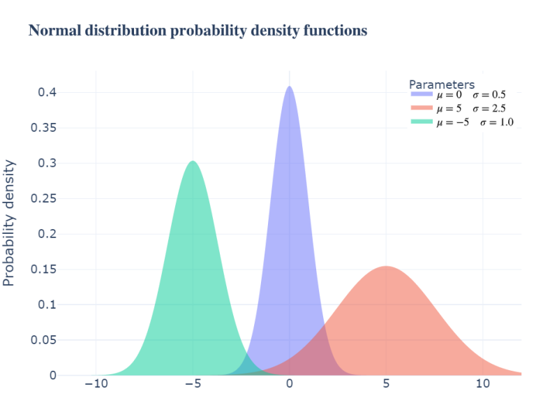
• The normal distribution which requires two parameters, mean (loc parameter in tfp) and standard deviation (scale parameter in tfp). To ensure that the predicted parameters produce a valid distribution, the standard deviations, which must be a positive value, are computed adding a little constant of 10-3 to the SoftPlus function of the predicted parameters.
def normal_distr(parameters):
return tfd.Normal(
loc = parameters[..., 0],
scale = 1e-3 + tf.math.softplus(parameters[..., 1]),
)
• The JohnsonSU distribution which requires four parameters, skewness, tail weight, mean (loc parameter in tfp) and sigma (scale parameter in tfp).
def jsu_distr(parameters):
return tfd.JohnsonSU(
skewness = parameters[..., 0],
tailweight = 1e-3 + tf.math.softplus(parameters[..., 1]),
loc = parameters[..., 2],
scale = 1e-3 + tf.math.softplus(parameters[..., 3]),
)
• A mixture of three normal distributions which requires a total of nine parameters, three for the means, three for the standard deviations and three for modelling the relative weight of each distribution. To compute the weights of the mixture distributions the SoftMax function is used with the predicted weights, thus ensuring that they sum to one and can be used as a probability.
def three_normal_mixture(parameters):
probs = tf.nn.softmax(parameters[..., :3])
locs = parameters[..., 3:6]
stds = 1e-3 + tf.math.softplus(parameters[..., 6:])
return tfd.MixtureSameFamily(
mixture_distribution = tfd.Categorical(
probs = probs
),
components_distribution = tfd.Normal(
loc = locs,
scale = stds
)
)
• A mixture of two JohnsonSU distributions requiring a total of ten parameter, four parameters for each distribution plus two parameters predicting the weight of each distribution.
def two_jsu_mixture(parameters):
probs = tf.nn.softmax(parameters[..., :2])
skewness = parameters[..., 2:4]
tailweights = 1e-3 + tf.math.softplus(parameters[..., 4:6])
locs = parameters[..., 6:8]
scales = 1e-3 + tf.math.softplus(parameters[..., 8:])
return tfd.MixtureSameFamily(
mixture_distribution = tfd.Categorical(probs = probs),
components_distribution = tfd.JohnsonSU(
skewness = skewness,
tailweight = tailweights,
loc = locs,
scale = scales,
)
)
To better understand the parameters of a normal distribution, we import the required libraries and then we define and call a function to plot the probability density of three normal distributions with different mean and standard deviations, using our previously defined normal_distr function.
def plot_example_distributions(parameters, distr_fn, title = ""):
fig = go.Figure()
x = np.linspace(-12, 12, 1000)
# We define the greek letter of the parameters
name = ["mu", "sigma"] if distr_fn == normal_distr else ["gamma", "delta"]
for i in range(parameters.shape[1]):
fig.add_trace(go.Scatter(
x=x,
y=distr_fn(parameters[..., i]).prob(x),
fill= 'tozeroy',
mode= 'none',
name = f"$\\{name[0]}={parameters[0][i]:.0f}\quad\\{name[1]}={parameters[1][i]:2}$"
))
# We style the titles and fonts for our plot
# The titles are defined using markdown for all the plots.
fig.update_layout(
title = f"$\large\\bf{{\\text{{{title}}}}}$",
legend_title = "Parameters",
yaxis_title = "Probability density",
legend=dict(
yanchor="top",
y=0.99,
xanchor="right",
x=0.99,
font=dict(
size=13,
color="black"
),
),
template = "plotly_white",
font = dict(size = 16),
height = 600,
width = 800
)
fig.show()
parameters = tf.constant(
[[0., 5., -5.], # We want three means; zero, five and minus five
[0.5, 2.5, 1.]] # For the standard deviations we define 0.5, 2.5 and 1.
)
plot_example_distributions(
parameters,
distr_fn = normal_distr,
title = "Normal distribution probability density functions")
To also visualize the JohnsonSU distribution, we call the previously defined function using the jsu_distr function and setting the mean to zero and sigma to one, to better understand the effect of the skewness and tailweigths parameters.
parameters = tf.constant(
[[-3, 2, 0.], # We define three values for the skewness
[1., 0.5, 0.25], # We define three different tailweights
[0.]*3, # We set the means to zero
[1.]*3]) # We set the sigmas to one
plot_example_distributions(parameters, jsu_distr,
title = "JohnsonSU distribution probability density functions")
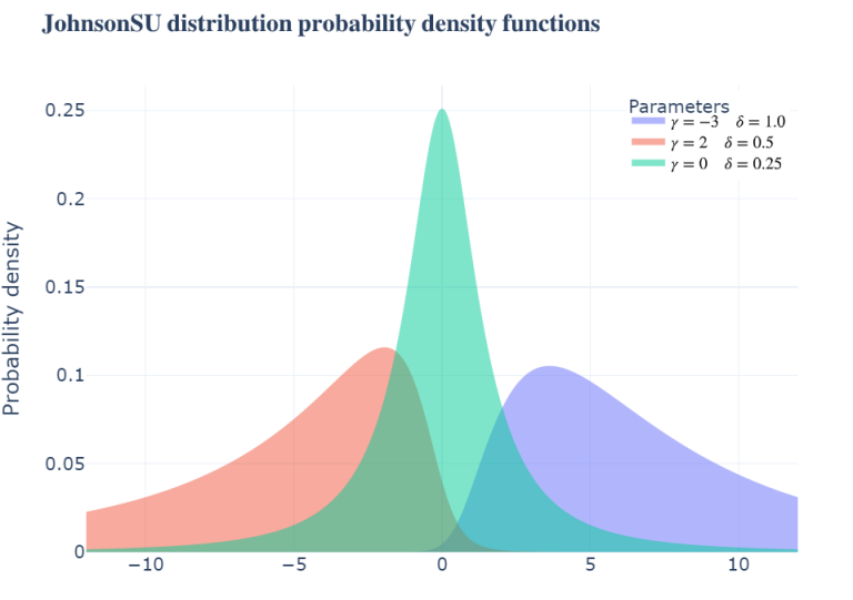
Although this distribution uses double the parameters of the normal distribution, it can clearly model more complex underlying distributions of data.
We will set the key for the API, this key is obtained using the Eikon APP to generate keys.
# The key is placed in a text file so that it may be used in this code without showing it itself:
eikon_key = open("eikon.txt","r")
ek.set_app_key(str(eikon_key.read()))
# It is best to close the files we opened in order to make sure that we don't stop any other services/programs from accessing them if they need to:
eikon_key.close()
The dates defined for the study are stored in the variable dates.
dates = pd.date_range('2002', '2020', freq = 'YS')
We define the required fields for our study, we want the date of announcement to know the day when the fundamentals were available. In addition, we define a dictionary to rename some of the columns and create an empty dataframe to store the data.
fields = [
"TR.F.OriginalAnnouncementDate", # Date of announcement
"TR.F.NetIncAfterTax", # Net income
"TR.F.IncBefTax", # Income before taxes
"TR.F.IncBefTaxtoEBIT", # Income before taxes to EBIT
"TR.F.EBITMargPct", # EBIT to revenues
"TR.F.TotRevBizActiv", # Revenue from business activities
"TR.F.TotAssets", # Total assets
"TR.F.ComEqTot", # Common total equity
"TR.F.DivPayoutRatioPct", # % Payout
]
columns = {
'Original Announcement Date Time': "pdate",
'52 Week Total Return': "y_return",
'YTD Total Return': "ytd"
}
df_full = pd.DataFrame()
We define a function that takes a dataframe and calculates the five variables of the DuPont Analysis of the ROE, which will be used later for our analysis. This function also rescales the input data for the neural network and then, it returns the dataframe containing a column storing the identifier of each company, the date of publication of results, the return for the following year, the five variables of DuPont and the dividend payout rate.
def normalize_data(df):
dupont_fields = [
"tax_burden",
"interest_burden",
"EBIT_margin",
"total_asset_turnover",
"leverage"
]
other_fields = ['Instrument', 'pdate',
'return', 'payout']
df["tax_burden"] = (df['Net Income after Tax'] /
df['Income before Taxes'])
df["interest_burden"] = df['Income before Taxes to EBIT']
df["EBIT_margin"] = df['EBIT Margin - %']/100
df["total_asset_turnover"] = (df['Revenue from Business Activities - Total'] /
df['Total Assets'])
df["leverage"] = (df['Total Assets'] /
df['Common Equity - Total'] / 100)
df["payout"] = df['Dividend Payout Ratio - %'] / 100
return df[other_fields + dupont_fields]
For each year, we obtain the fundamentals of that year, the total returns of that stock for the following year and the total returns during the month of January. We will study only those companies whose publication of results took place in January, thus we will discard the few companies that publish results afterwards. Therefore, we only want to obtain the results since February (once the fundamental information is already available for the selected companies), which is done by subtracting the returns of January from the total returns of that year.
for date in dates:
year = int(str(date.to_period('Y')))
# We define three dictionaries containing the parameters
# One for the fundamental data reported that year
params = {'SDate': f"{year}-01-01",
"EDate": f"{year}-12-31",
"Frq": "FY"}
# Another for the returns of the following year
params_future = f'SDate={year+1}-01-01,EDate={year+1}-12-31'
# The last one for obtaining the returns up to February
params_feb = f'SDate={year+1}-02-01,EDate={year+1}-02-01'
# We define the return fields
0
future_return = [
f"TR.TotalReturn52Wk({params_future})",
f"TR.TotalReturnYTD({params_feb})"
]
# This function helps cleaning the data
def data_cleaning(row):
row = row.split('T')[0]
return row if int(row[:4])>=year else np.nan
# Finally we obtain the data and call the previously defined functions
# In addition, the data is prepared and appended to the defined dataframe
df = ek.get_data(f'0#.SPXBK({date.to_period("D")})',
fields + future_return, params)[0]
# 0#.SPXBK is the code to obtain the financial companies of the S&P500
# ({date.to_period("D")}) specifies that we are interested in the constituents
# at the starting of that year.
df = df.replace('', np.nan).dropna().rename(columns = columns)
df["pdate"] = pd.to_datetime(df["pdate"].apply(data_cleaning))
df["return"] = (df["y_return"].astype(np.float32) -
df["ytd"].astype(np.float32))
df = normalize_data(df).dropna()
df_full = df_full.append(df)
Here we save only the companies whose publication date took place in January
df_full = df_full[df_full["pdate"].dt.month == 1]
Now that we have a dataframe containing one row for each year of a company data, we want to obtain another dataframe containing the daily returns of each company in the previously filled dataframe. Moreover, we want to add the fundamental data to the daily returns of the stock, thus allowing for easier training of the neural networks that will be defined later. We use the open for computing the returns because the close would not be known at that day, thus it only uses the available information at market open, when it would still be possible to take a trading decision.
# First we store the columns containing the fundamental data
columns = [column for column in df_full.columns if column not in ["pdate", "return", "Instrument"]]
# Then, we store the name of the companies and the dates after the date of publication
stocks = df_full["Instrument"]
starts = (df_full["pdate"] + pd.Timedelta("1D")).astype(str)
features = df_full[columns].values
df_ts = pd.DataFrame() # We will fill this dataframe with all the data
# This function takes a date as input and returns that date for the next year
def end(date):
ending = pd.to_datetime(date) + pd.Timedelta("365D")
return str(ending.to_period("D"))
# For each company, we obtain a year of daily "Open" data, we add our fundamental
# variables for that year to the dataframe, we calculate the daily percentage
# change of the open of that stock and we store the results in df_ts.
for stock, start, feature in zip(stocks,starts, features):
df = ek.get_timeseries(stock, ['OPEN'],
start_date=start,
end_date = end(start),
interval = "daily")
df["target"] = 100*df["OPEN"].pct_change().astype(np.float32)
df["stock"] = stock
df[columns] = feature
df.index = pd.to_datetime(df.index)
# We create a multiindex dataframe appending
# the identifier of the stock to the dates index.
df = df.set_index("stock", append = True)
df_ts = df_ts.append(df.dropna().drop("OPEN", axis = 1))
# Finally we sort the data by its index
df_ts = df_ts.sort_index()
We set the date as index of our first created dataframe and convert the numerical columns to the np.float32 dtype.
df_full = df_full.set_index("pdate").sort_index()
for column in df_full.columns:
try: df_full[column] = df_full[column].astype(np.float32)
except: continue
Here, we define the negative log likelihood, which is then used as the loss of our models. This is the standard loss function used for probabilistic models and computing it is very easy to compute with tensorflow_probability.
NLL = lambda y, distr: -distr.log_prob(y)
For training the neural network we store the data from 2002 to 2011, both years included. The features are the six variables that were previously defined and the target is the daily percentage of change of the open price of the company. For validation data we use the dates from 2012 to 2015, both years included. Finally, to test our neural networks we store the data since 2016 in the test variables.
X_train, y_train = df_ts.loc[:"2011"].drop("target", axis = 1), df_ts.loc[:"2011"].pop("target")
X_val, y_val = df_ts.loc["2012":"2015"].drop("target", axis = 1), df_ts.loc["2012":"2015"].pop("target")
X_test, y_test = df_ts.loc["2016":].drop("target", axis = 1), df_ts.loc["2016":].pop("target")
Here we define two auxiliary functions, the first one creates a neural network made of one batch normalization layer (Ioffe and Szegedy, 2015) followed by two fully connected layers of 32 neurons each, with exponential linear unit activations (Clevert, Unterthiner and Hochreiter, 2016) and with one batch normalization layer in between. After these layers there is another fully connected layer, which returns the parameters required to model the distribution. Finally, those parameters are used to create a distribution from which to compute the loss during training.
The second function takes a model and data containing the features and returns the predicted parameters of the distribution. Given that the last layer of our models is a probability distribution, calling the predict method of these models returns a random sample from the predicted distribution. However, by returning the predicted parameters we can create the predicted distribution, which allows us to investigate further.
def get_model(distr, n_params):
neurons = 32
inputs = layers.Input(shape = (X_train.shape[1],))
x = layers.BatchNormalization()(inputs)
x = layers.Dense(neurons,
activation = "elu")(inputs)
x = layers.BatchNormalization()(x)
x = layers.Dense(neurons,
activation = "elu")(x)
x = layers.Dense(n_params)(x)
outputs = tfp.layers.DistributionLambda(distr)(x)
model = tf.keras.models.Model(inputs = inputs, outputs = outputs)
return model
def get_parameters(model, X):
p_model = tf.keras.models.Model(
inputs = model.inputs,
outputs = model.layers[-2].output
)
return p_model.predict(X)
Now, we define some options for training the models. In particular the neural networks are trained using the Adam optimizer (Kingma and Ba, 2017) with a starting learning rate of 0.05, which is divided by two after a stagnation of the training loss for five epochs in a row. In addition, the training is stopped when the validation loss does not improve for a hundred consecutive epochs, returning to the weights obtained when the validation loss reached its minimum.
optimizer = tf.optimizers.Adam(5e-2)
my_distributions = [
normal_distr,
jsu_distr,
three_normal_mixture,
two_jsu_mixture,
]
n_params = [2, 4, 9, 10]
early_stop = tf.keras.callbacks.EarlyStopping(
monitor='val_loss',
patience=30,
verbose=0,
restore_best_weights=True
)
reduce_lr = tf.keras.callbacks.ReduceLROnPlateau(
monitor='loss',
factor=0.25,
patience=4,
verbose=0
)
Finally, we create our models and store them in a list. Moreover, we create two empty lists to store the results during training and the results in the test set of each model. After compiling each model, using the previously defined optimizer and loss, we train the models, then we predict the parameters of the distributions of returns of each company for each year in the test set. Then, we create the predicted distributions and store the loss in the test set in our list.
models = [get_model(d, n) for (d, n) in zip(my_distributions, n_params)]
history = []
test_loss = []
for distr, model in zip(my_distributions, models):
model.compile(optimizer = optimizer, loss = NLL)
# This step can take a few minutes to complete, given the use of some random
# variables it can produce significantly different results between runs.
# Sometimes the predicted parameters might even result in some null values for some
# of the distributions under some rare initializations of the neural networks
history.append(
model.fit(
X_train,
y_train,
epochs = 1000,
validation_data=(X_val, y_val),
batch_size = 512,
verbose = 0, # This value can be increased to visualize the progress.
callbacks = [early_stop, reduce_lr]
)
)
parameters = get_parameters(model, X_test)
dist = distr(parameters)
test_loss.append(tf.reduce_mean(NLL(y_test, dist)))
Here, we transform the predicted distributions to two values, one for those companies whose predicted distribution's mean divided by its standard deviation is higher than the mean and zero for the rest. These values will be stored in the df_full dataframe as columns. To avoid printing the warnings that might be produced using this method we import the warnings library to ignore them. In addition, we store the predicted distributions in a list, for plotting them later.
import warnings
plotting_distributions = []
X_full = df_full.drop(["Instrument", "return"], axis = 1)
for i, model in enumerate(models):
parameters = get_parameters(model, X_full)
dist = my_distributions[i](parameters)
df_full[f"prediction_model_{i}"] = tf.reshape(
dist.mean()/dist.stddev(),
shape = [-1])
plotting_distributions.append([my_distributions[i](p) for p in parameters])
quantiles = pd.Series(dtype = np.float32)
quantiles_mean = pd.Series(dtype = np.float32)
n_quantiles = 2
for date in dates:
with warnings.catch_warnings():
warnings.simplefilter("ignore")
quantiles = quantiles.append(
pd.qcut(
df_full[f"prediction_model_{i}"].loc[str(date.year)],
n_quantiles,
labels = False,
duplicates='drop'
)
)
df_full[f"value_{i}"] = quantiles
We store the names of our models in a list and show the results on the test set by accessing the previously defined list test_loss, which stores the neg log likelihood for the four distributions. The lower this loss, the better the observed results were described with the predicted distribution.
model_names = ["Normal distribution", "JohnsonSU distribution", "Mixture of normals", "Mixture of JohnsonSU"]
for i, model in enumerate(model_names):
print(f"The test loss for the {model} model was {test_loss[i].numpy():.3f}.")
The test loss for the Normal distribution model was 2.233.
The test loss for the JohnsonSU distribution model was 7.631.
The test loss for the Mixture of normals model was 2.440.
The test loss for the Mixture of JohnsonSU model was 2.088.
In addition we print the returns obtained with our defined method for each model in the test set.
for i,_ in enumerate(my_distributions):
top_value = df_full["return"][df_full[f"value_{i}"] == (n_quantiles-1)].loc["2016":].mean()
bot_value = df_full["return"][df_full[f"value_{i}"] == 0].loc["2016":].mean()
print(f"{(top_value - bot_value)*100 :.0f} BPS each year with the {model_names[i]} model.")
367 BPS each year with the Normal distribution model.
nan BPS each year with the JohnsonSU distribution model.
-102 BPS each year with the Mixture of normals model.
172 BPS each year with the Mixture of JohnsonSU model.
During the test set period, the mean returns of all the companies under analysis is shown below:
mean_BPS = df_full['return'].loc['2016':].mean()*100
print(f"The mean return of the companies in the test set was {mean_BPS:.0f} BPS each year")
The mean return of the companies in the test set was 650 BPS each year
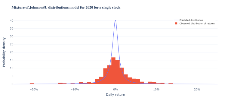
Now we will define a function to plot the predicted distribution for a given stock in our dataset for the year 2020. In particular, the function is called to plot the last stock in the dataset and the predicted mixture of JohnsonSU distribution compared with the observer distribution of returns.
x = np.linspace(-0.25, 0.25, 1000)
def plot_distribution(number = 0, title = "", stock = -1):
fig = go.Figure(go.Scatter(x = x,
y = 100*plotting_distributions[number][stock].prob(x*100),
mode = "lines",
name = "Predicted distribution"
))
fig.add_trace(go.Histogram(
x=df_ts.loc[slice("2020", None), df_ts.index[stock][1], :]["target"]/100,
histnorm='probability density',
name = "Observed distribution of returns"
))
fig.update_layout(
title = f"$\large\\bf{{\\text{{{title}}}}}$",
xaxis_title = "Daily return",
yaxis_title = "Probability density",
legend=dict(
yanchor="top",
y=0.99,
xanchor="right",
x=0.99,
font=dict(
size=13,
color="black"
),
),
xaxis = dict(tickformat = '%'),
template = "plotly_white",
font = dict(size = 16),
height = 600,
width = 800
)
fig.show()
plot_distribution(number = 3, title = "Mixture of JohnsonSU distributions model for 2020 for a single stock", stock = -1)
To also visualize the training and validation losses we plot them using the previously defined history variable which stores the metrics of our models during training.
fig = go.Figure()
for i, name in enumerate(model_names):
fig.add_trace(go.Scatter(
x = np.arange(len(history[i].history["loss"])),
y = history[i].history["loss"],
mode = "lines",
name = f"Training loss {name}"
))
fig.add_trace(go.Scatter(
x = np.arange(len(history[i].history["val_loss"])),
y = history[i].history["val_loss"],
mode = "lines",
name = f"Validation loss {name}"
))
fig.update_layout(
title = r"$\large\bf{\text{Losses during the training phase}}$",
legend=dict(
yanchor="top",
y=0.99,
xanchor="right",
x=0.99,
font=dict(
size=13,
color="black"
),
),
xaxis_title = "Epochs",
yaxis_title = "Negative log likelihood",
template = "plotly_white",
font = dict(size = 16),
height = 600,
width = 800
)
fig.show()
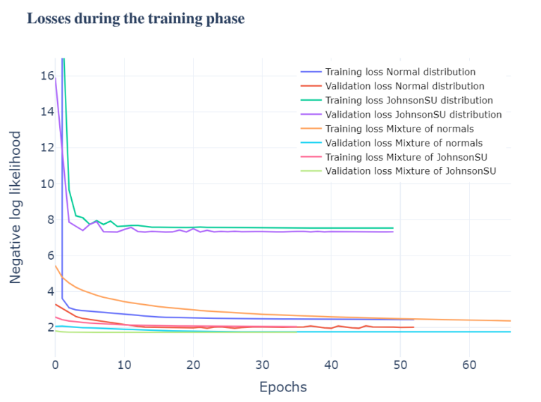
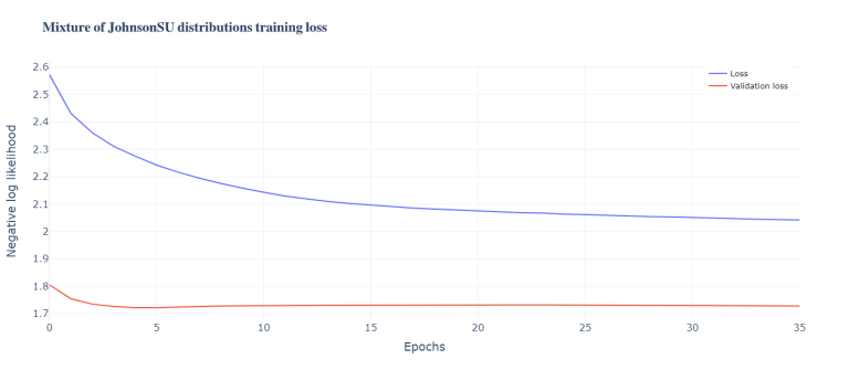
In addition, another function is defined to plot the loss of each individual model to better visualize these losses. It can be seen that the training loss and the validation almost go in parallel. In this case we call the function to plot the losses of the mixture of JohnsonSU distributions model.
def plot_model_loss(number = 0, title = ""):
fig = go.Figure(go.Scatter(
x = np.arange(len(history[number].history["loss"])),
y = history[number].history["loss"],
mode = "lines",
name = "Loss"
))
fig.add_trace(go.Scatter(
x = np.arange(len(history[number].history["val_loss"])),
y = history[number].history["val_loss"],
mode = "lines",
name = "Validation loss"
))
fig.update_layout(
title = f"$\large\\bf{{\\text{{{title}}}}}$",
xaxis_title = "Epochs",
yaxis_title = "Negative log likelihood",
legend=dict(
yanchor="top",
y=0.99,
xanchor="right",
x=0.99,
font=dict(
size=13,
color="black"
),
),
template = "plotly_white",
font = dict(size = 16),
height = 600,
width = 800
)
fig.show()
plot_model_loss(3, title = "Mixture of JohnsonSU distributions training loss")
4. Conclusions
The proposed approach offers two advantages compared with other deep learning structures. On the one hand, it allows to train more parameters without overfitting to the data as it can be trained on higher frequencies. On the other hand, it allows for more informed decisions as there is a predicted probability of returns. The method of RPV shows an example of using returns distributions for selecting stocks.
However, this method also has some drawbacks. The subjective choice of the distribution influences the predicted results. Moreover, the initialization of the weights acquires greater importance compared with other models.
In conclusion, this model produces more informative outputs, although it comes with the price of added complexity for training. Further investigation could lead to improved results using other frequencies of returns or even tick data. In addition, a smarter initialization of the weights could achieve convergence in a more consistent manner.
Future lines of work
The choice of the underlying distribution has a significant effect on the results, thus it requires further investigation and testing of different distributions. Some possible solutions for this aspect are choosing more flexible distributions thus reducing the importance of this subjective decision, as it allows the neural network to model more complex distributions of returns. In this line, normalizing flows (Kobyzev, Prince and Brubaker, 2020) seem to offer another solution to model distributions, being a possible alternative.
This paper used six variables as input for the neural network, however the model could benefit from using more variables or making use of higher frequency data.
Finally, although only the financial sector was studied, other sectors could be analysed using the proposed RPV model given that the input variables are not sector specific. In this sense, this could be applied to all the companies across sectors to predict its distributions of returns.
Bibliography
Chong, E., Han, C. and Park, F.C., 2017. Deep learning networks for stock market analysis and prediction: Methodology, data representations, and case studies. Expert Systems with Applications, 83, pp.187–205.
Clevert, D.-A., Unterthiner, T. and Hochreiter, S., 2016. Fast and Accurate Deep Network Learning by Exponential Linear Units (ELUs). arXiv:1511.07289 [cs]. [online] Available at: http://arxiv.org/abs/1511.07289 [Accessed 31 Jan. 2021].
Feng, G., He, J. and Polson, N.G., 2018. Deep Learning for Predicting Asset Returns. arXiv:1804.09314 [cs, econ, stat]. [online] Available at: http://arxiv.org/abs/1804.09314 [Accessed 3 Feb. 2021].
Fischer, T. and Krauss, C., 2018. Deep learning with long short-term memory networks for financial market predictions. European Journal of Operational Research, 270(2), pp.654–669.
Ioffe, S. and Szegedy, C., 2015. Batch Normalization: Accelerating Deep Network Training by Reducing Internal Covariate Shift. arXiv:1502.03167 [cs]. [online] Available at: http://arxiv.org/abs/1502.03167 [Accessed 3 Feb. 2021].
Kingma, D.P. and Ba, J., 2017. Adam: A Method for Stochastic Optimization. arXiv:1412.6980 [cs]. [online] Available at: http://arxiv.org/abs/1412.6980 [Accessed 3 Feb. 2021].
Kobyzev, I., Prince, S. and Brubaker, M., 2020. Normalizing Flows: An Introduction and Review of Current Methods. IEEE Transactions on Pattern Analysis and Machine Intelligence, pp.1–1.
Lachiheb, O. and Gouider, M.S., 2018. A hierarchical Deep neural network design for stock returns prediction. Procedia Computer Science, 126, pp.264–272.
Li, W. and Mei, F., 2020. Asset returns in deep learning methods: An empirical analysis on SSE 50 and CSI 300. Research in International Business and Finance, 54, p.101291.
Wang, J., Sun, T., Liu, B., Cao, Y. and Wang, D., 2018. Financial Markets Prediction with Deep Learning. In: 2018 17th IEEE International Conference on Machine Learning and Applications (ICMLA). 2018 17th IEEE International Conference on Machine Learning and Applications (ICMLA). pp.97–104.
Related Articles