
Only quarterly USA GDP data is published; this article describes a method of estimating monthly such figures using monthly Total Compensation figures.
Introduction
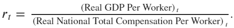
Gross Domestic Product (GDP) is often thought of and calculated with an Expenditure Approach such that GDP=C+I+G+(X−M) where C = Consumption, I = Investment, G = Government Spending, & (X–M) = Net Exports, but it is also possible to calculate it via a per worker Income Approach. With this approach, we may estimate GDP Per Worker (GDPPW) with Total Compensation Per Worker (TCPW) figures such that (as per Appendix 1):

where
We can then attempt to interpolate GDPPW values at higher frequencies than they are officially released with higher wage/income figure releases (exempli gratia (e.g.): to compute monthly GDP figures when only quarterly ones are released using monthly published Total Compensation data).
We have to be careful of a few difficulties outlined by Feldstein (2008) (MF hereon): "The relation between productivity [ id est (i.e.): GDP] and wages has been a source of substantial controversy, not only because of its inherent importance but also because of the conceptual measurement issues that arise in making the comparison." (Feldstein (2008)). MF outlines several key factors (KF hereon) to consider when studying the question:
- "[An undeserved] focus on wages rather than total compensation. Because of the rise in fringe benefits and other noncash payments, wages have not risen as rapidly as total compensation. It is important therefore to compare the productivity rise with the increase of total compensation rather than with the increase of the narrower measure of just wages and salaries.” This is why this article will first focus on using Total Compensation (TC).
- “[… The] nominal compensation deflated by the CPI is not appropriate for evaluating the relation between productivity and compensation […] this implies that the real marginal product of labor should be compared to the wage deflated by the product price and not by some consumer price index. [...] The CPI differs from the nonfarm product price in several ways. The inclusion in the CPI, but not in the nonfarm output price index, of the prices of imports and of the services provided by owner occupied homes is particularly important." This is why this article will first focus on using Nominal T.C. deflated (made 'real') with the Nonfarm Business Sector Output Price Index Deflator (NBSOPID).
Keeping these points in mind, we will attempt to investigate the relationship between the United States of America( U.S.A.)'s Real GDP (RGDP) and U.S.A.'s Real National Total Compensation (RNTC) in order to construct a framework allowing us to estimate monthly RGDP data when only quarterly data is published.
Numerical Approximation
Background
As per Appendix 1:
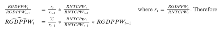
It may seem needlessly convoluted to insert 𝑟𝑡 the way it was done above, but it was necessary due to the fact that we have 𝑟𝑡rt estimates (𝑟𝑡ˆ) - we thus build our framework around it: since Total Compensation figures are released on a monthly basis, if we can construct an estimate for the linearly-time-variant 𝑟𝑡rt, we can then construct monthly GDP figures (even though only quarterly ones are published).
This article will study the efficiency of the USA Real GDP Per Worker To National Real Total Compensation Per Worker Ratio (RGDPPWTNRTCPWR) as the ratio '𝑟𝑡'.
Development Tools & Resources
The example code demonstrating the use case is based on the following development tools and resources:
- Refinitiv's DataStream Web Services (DSWS): Access to DataStream data. A DataStream or Refinitiv Workspace IDentification (ID) will be needed to run the code bellow.
- Python Environment: Tested with Python 3.7
- Packages: DatastreamDSWS, Numpy, Pandas, statsmodel, scipy and Matplotlib. The Python built in modules statistics, datetime and dateutil are also required.
Import libraries
# The ' from ... import ' structure here allows us to only import the
# module ' python_version ' from the library ' platform ':
from platform import python_version
print("This code runs on Python version " + python_version())
This code runs on Python version 3.7.4
We need to gather our data. Since Refinitiv's DataStream Web Services (DSWS) allows for access to the most accurate and wholesome end-of-day (EOD) economic database (DB), naturally it is more than appropriate. We can access DSWS via the Python library "DatastreamDSWS" that can be installed simply by using pip installpip install.
import DatastreamDSWS as DSWS
# We can use our Refinitiv's Datastream Web Socket (DSWS) API keys that allows us to be identified by
# Refinitiv's back-end services and enables us to request (and fetch) data:
# The username is placed in a text file so that it may be used in this code without showing it itself:
DSWS_username = open("Datastream_username.txt","r")
# Same for the password:
DSWS_password = open("Datastream_password.txt","r")
ds = DSWS.Datastream(username = str(DSWS_username.read()), password = str(DSWS_password.read()))
# It is best to close the files we opened in order to make sure that we don't stop any other
# services/programs from accessing them if they need to:
DSWS_username.close()
DSWS_password.close()
The following are Python-built-in module/library, therefore it does not have a specific version number.
import os # os is a library used to manipulate files on machines
import datetime # datetime will allow us to manipulate Western World dates
import dateutil # dateutil will allow us to manipulate dates in equations
import warnings # warnings will allow us to manupulate warning messages (such as depretiation messages)
statistics, numpy, scipy and statsmodels are needed for datasets' statistical and mathematical manipulations
import statistics # This is a Python-built-in module/library, therefore it does not have a specific version number.
import numpy
import statsmodels
from statsmodels.tsa.api import ExponentialSmoothing, SimpleExpSmoothing, Holt
import scipy
from scipy import stats
for i,j in zip(["numpy", "statsmodels", "scipy"], [numpy, statsmodels, scipy]):
print("The " + str(i) + " library imported in this code is version: " + j.__version__)
The numpy library imported in this code is version: 1.16.5
The statsmodels library imported in this code is version: 0.10.1
The scipy library imported in this code is version: 1.3.1
pandas will be needed to manipulate data sets
import pandas
pandas.set_option('display.max_columns', None) # This line will ensure that all columns of our dataframes are always shown
print("The pandas library imported in this code is version: " + pandas.__version__)
The pandas library imported in this code is version: 0.25.1
matplotlib is needed to plot graphs of all kinds
import matplotlib
import matplotlib.pyplot as plt
print("The matplotlib library imported in this code is version: "+ matplotlib.__version__)
The matplotlib library imported in this code is version: 3.1.1
def Translate_to_First_of_the_Month(data, dataname):
"""This function will put Refinitiv's DataStream data into a Pandas Dafaframe
and normalise it to the 1st of the month it was collected in."""
# The first 8 characters of the index is the ' yyyy-mm- ', onto which will be added '01':
data.index = data.index.astype("str").str.slice_replace(8, repl = "01")
data.index = pandas.to_datetime(data.index)
data.columns = [dataname]
return data
The cell below defines a function that appends our monthly data-frame with chosen data
df = pandas.DataFrame([])
def Add_to_df(data, dataname):
global df # This allows the function to take the pre-deffined variable ' df ' for granted and work from there
DS_Data_monthly = Translate_to_First_of_the_Month(data, dataname)
df = pandas.merge(df, DS_Data_monthly,
how = "outer",
left_index = True,
right_index=True)
# Using an implicitly registered datetime converter for a matplotlib plotting method is no
# longer supported by matplotlib. Current versions of pandas requires explicitly
# registering matplotlib converters.
pandas.plotting.register_matplotlib_converters()
def Plot1ax(dataset, ylabel = "", title = "", xlabel = "Year", datasubset = [0],
datarange = False, linescolor = False, figuresize = (12,4),
facecolor = "0.25", grid = True):
""" Plot1ax Version 1.0:
This function returns a Matplotlib graph with default colours and dimensions
on one y axis (on the left as oppose to two, one on the left and one on the right).
datasubset (list): Needs to be a list of the number of each column within
the data-set that needs to be labelled on the left.
datarange (bool): If wanting to plot graph from and to a specific point,
make datarange a list of start and end date.
linescolor (bool/list): (Default: False) This needs to be a list of the color of each
vector to be ploted, in order they are shown in their data-frame from left to right.
figuresize (tuple): (Default: (12,4)) This can be changed to give graphs of different
proportions. It is defaulted to a 12 by 4 (ratioed) graph.
facecolor (str): (Default: "0.25") This allows the user to change the
background color as needed.
grid (bool): (Default: "True") This allows us to decide whether or
not to include a grid in our graphs.
"""
if datarange == False:
start_date = str(dataset.iloc[:,datasubset].index[0])
end_date = str(dataset.iloc[:,datasubset].index[-1])
else:
start_date = str(datarange[0])
if datarange[-1] == -1:
end_date = str(dataset.iloc[:,datasubset].index[-1])
else:
end_date = str(datarange[-1])
fig, ax1 = plt.subplots(figsize = figuresize, facecolor = facecolor)
ax1.tick_params(axis = 'both', colors = 'w')
ax1.set_facecolor(facecolor)
fig.autofmt_xdate()
plt.ylabel(ylabel, color = 'w')
ax1.set_xlabel(str(xlabel), color = 'w')
if linescolor == False:
for i in datasubset: # This is to label all the lines in order to allow matplot lib to create a legend
ax1.plot(dataset.iloc[:, i].loc[start_date : end_date],
label = str(dataset.columns[i]))
else:
for i in datasubset: # This is to label all the lines in order to allow matplot lib to create a legend
ax1.plot(dataset.iloc[:, i].loc[start_date : end_date],
label = str(dataset.columns[i]),
color = linescolor)
ax1.tick_params(axis='y')
if grid == True:
ax1.grid(color='black', linewidth = 0.5)
ax1.set_title(str(title) + " \n", color='w')
plt.legend()
plt.show()
The cell below defines a function to plot data on two y axis.
def Plot2ax(dataset, rightaxisdata, y1label, y2label, leftaxisdata,
title = "", xlabel = "Year", y2color = "C1", y1labelcolor = "C0",
figuresize = (12,4), leftcolors = ('C1'), facecolor = "0.25"):
""" Plot2ax Version 1.0:
This function returns a Matplotlib graph with default colours and dimensions
on two y axis (one on the left and one on the right)
leftaxisdata (list): Needs to be a list of the number of each column within
the data-set that needs to be labelled on the left
figuresize (tuple): (Default: (12,4)) This can be changed to give graphs of
different proportions. It is defaulted to a 12 by 4 (ratioed) graph
leftcolors (str / tuple of (a) list(s)): This sets up the line color for data
expressed with the left hand y-axis. If there is more than one line,
the list needs to be specified with each line colour specified in a tuple.
facecolor (str): (Default: "0.25") This allows the user to change the
background color as needed
"""
fig, ax1 = plt.subplots(figsize=figuresize, facecolor=facecolor)
ax1.tick_params(axis = "both", colors = "w")
ax1.set_facecolor(facecolor)
fig.autofmt_xdate()
plt.ylabel(y1label, color=y1labelcolor)
ax1.set_xlabel(str(xlabel), color = "w")
ax1.set_ylabel(str(y1label))
for i in leftaxisdata: # This is to label all the lines in order to allow matplot lib to create a legend
ax1.plot(dataset.iloc[:, i])
ax1.tick_params(axis = "y")
ax1.grid(color='black', linewidth = 0.5)
ax2 = ax1.twinx() # instantiate a second axes that shares the same x-axis
color = str(y2color)
ax2.set_ylabel(str(y2label), color=color) # we already handled the x-label with ax1
plt.plot(dataset.iloc[:, list(rightaxisdata)], color=color)
ax2.tick_params(axis='y', labelcolor='w')
ax1.set_title(str(title) + " \n", color='w')
fig.tight_layout() # otherwise the right y-label is slightly clipped
plt.show()
The cell below defines a function to plot data regressed on time.
def Plot_Regression(x, y, slope, intercept, ylabel,
title="", xlabel="Year", facecolor="0.25", data_point_type = ".", original_data_color = "C1",
time_index = [], time_index_step = 48, figuresize = (12,4), line_of_best_fit_color = "b"):
""" Plot_Regression Version 1.0:
Plots the regression line with its data with appropriate default Refinitiv colours.
facecolor (str): (Default: "0.25") This allows the user to change the background color as needed
figuresize (tuple): (Default: (12,4)) This can be changed to give graphs of different proportions. It is defaulted to a 12 by 4 (ratioed) graph
line_of_best_fit_color (str): This allows the user to change the background color as needed.
' time_index ' and ' time_index_step ' allow us to dictate the frequency of the ticks on the x-axis of our graph.
"""
fig, ax1 = plt.subplots(figsize = figuresize, facecolor = facecolor)
ax1.tick_params(axis = "both", colors = "w")
ax1.set_facecolor(facecolor)
fig.autofmt_xdate()
plt.ylabel(ylabel, color = "w")
ax1.set_xlabel(xlabel, color = "w")
ax1.plot(x, y, data_point_type, label='original data', color = original_data_color)
ax1.plot(x, intercept + slope * x, "r", label = "fitted line", color = line_of_best_fit_color)
ax1.tick_params(axis = "y")
ax1.grid(color='black', linewidth = 0.5)
ax1.set_title(title + " \n", color='w')
plt.legend()
if len(time_index) != 0:
# locs, labels = plt.xticks()
plt.xticks(numpy.arange(len(y), step = time_index_step),
[i for i in time_index[0::time_index_step]])
plt.show()
Setup Statistics Tools
def Single_period_Geometric_Growth(data):
""" This function returns the geometric growth of the data
entered at the frequency it is given. id est (i.e.): if
daily data is entered, a daily geometric growth rate is returned.
data (list): list including inc/float data recorded at a specific
frequency.
"""
data = list(data)
# note that we use ' len(data) - 1 ' instead of ' len(data) ' as the former already lost its degree of freedom just like we want it to.
single_period_geometric_growth = ( (data[-1]/data[0])**(1/((len(data))-1)) ) - 1
return single_period_geometric_growth
The cell below defines a function that creates and displays a table of statistics for all vectors (columns) within any two specified datasets.
def Statistics_Table(dataset1, dataset2 = ""):
""" This function returns a table of statistics for the one or two pandas
data-frames entered, be it ' dataset1 ' or both ' dataset1 ' and ' dataset2 '.
"""
Statistics_Table_Columns = list(dataset1.columns)
if str(dataset2) != "":
[Statistics_Table_Columns.append(str(i)) for i in dataset2.columns]
Statistics_Table = pandas.DataFrame(columns = ["Mean",
"Mean of Absolute Values",
"Standard Deviation",
"Median", "Skewness",
"Kurtosis",
"Single Period Growth Geometric Average"],
index = [c for c in Statistics_Table_Columns])
def Statistics_Table_function(data):
for c in data.columns:
Statistics_Table["Mean"][str(c)] = numpy.mean(data[str(c)].dropna())
Statistics_Table["Mean of Absolute Values"][str(c)] = numpy.mean(abs(data[str(c)].dropna()))
Statistics_Table["Standard Deviation"][str(c)] = numpy.std(data[str(c)].dropna())
Statistics_Table["Median"][str(c)] = numpy.median(data[str(c)].dropna())
Statistics_Table["Skewness"][str(c)] = scipy.stats.skew(data[str(c)].dropna())
Statistics_Table["Kurtosis"][str(c)] = scipy.stats.kurtosis(data[str(c)].dropna())
if len(data[str(c)].dropna()) != 1 or data[str(c)].dropna()[0] != 0: # This if statement is needed in case we end up asking for the computation of a value divided by 0.
Statistics_Table["Single Period Growth Geometric Average"][str(c)] = Single_period_Geometric_Growth(data[str(c)].dropna())
Statistics_Table_function(dataset1)
if str(dataset2) != "":
Statistics_Table_function(dataset2)
return Statistics_Table
USA Working Population Growth
We will use Yearly Geometric Growth rate when looking at geometric growth rates throughout this article, as outlined in Appendix 2.
We proportion of population which works. This includes only employed adults, excluding children (~ 20% of USAP) and the elderly (~ 14% of USAP). The cell below adds the United States of America's Working Population (USAWP) values to the data-frame 'df' and plots our population data this far:
df = Translate_to_First_of_the_Month(data = ds.get_data(tickers = 'USEMPTOTO', fields = "X", start = '1950-01-01', freq = 'M') * 1000,
dataname = "USAWP (monthly data)")
Next we take the USA Working Population's first Difference, i.e.: 𝑈𝑆𝐴𝑊𝑃𝐷𝑡=𝑈𝑆𝐴𝑊𝑃𝑡−𝑈𝑆𝐴𝑊𝑃𝑡−1
USAWPD = pandas.DataFrame(df["USAWP (monthly data)"].diff())
USAWPD.rename(columns = {'USAWP (monthly data)':'USAWPD (monthly data)'}, inplace = True)
df = pandas.merge(df, USAWPD, how = 'outer', left_index = True, right_index = True)
USA's Working Population's single period (in this case: monthly) Geometric Growth is then defined as USAWPG as per Appendix 2:
# Create our USAWPYGG (note that due to the use of logarythms in the scipy.stats.gmean function/class, we cannot use it here without yeilding an error)
USAWPYGG = ((1 + Single_period_Geometric_Growth(data = df["USAWP (monthly data)"].dropna()) )**12)-1
df["USAWPG (monthly data)"] = df["USAWPD (monthly data)"] / df["USAWP (monthly data)"]
Plot2ax(title = "USA Working Population (in blue) and its Growth (in orange) (USAWP & USAWPG) over the years (monthly data)",
dataset = df, leftaxisdata = [-3], rightaxisdata = [-1], y1label = "USAWP", y2label = "USAWPG", leftcolors = "w")
print("Our U.S.A.'s Working Population' Yearly Geometric Growth is " + str(USAWPYGG) + ", i.e.: " + str(USAWPYGG*100) + "%")
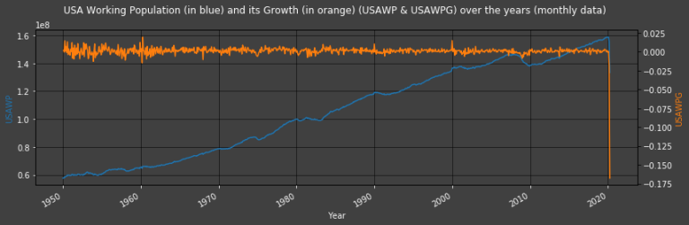
Our U.S.A.'s Working Population' Yearly Geometric Growth is 0.012018187303719507, i.e.: 1.2018187303719507%
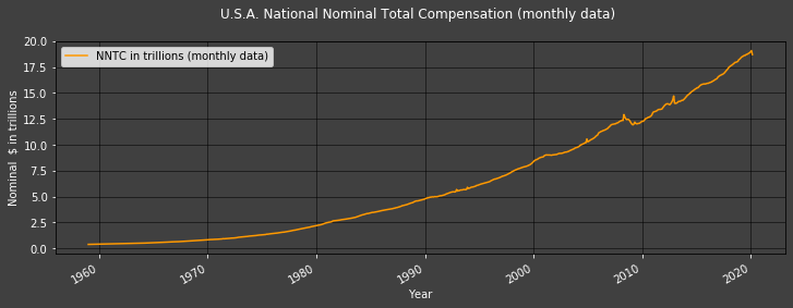
Total Compensation
As per MF's first KF, we use USA Nominal National Total Compensation (NNTC) - the nominal value of which is derived from National Nominal Personal Income Accounts. Note that this dataset is the inflows into accounts; this means that we do not need to include incomes from assets. Note also that deflators used to compute 'real' figures form 'nominal' are defined in Appendix 3.
National Nominal Total Compensation
We can now add out National Nominal Total Compensation (NNTC) data in our data-frame and plot if for good measure.
Add_to_df(data = ds.get_data(tickers = "USPERINCB",
fields = "X",
start = '1950-01-01', freq = 'M').dropna() * 1000000000,
dataname = "NNTC (monthly data)")
df["NNTC in trillions (monthly data)"] = df["NNTC (monthly data)"] / 1000000000000
Plot1ax(title = "U.S.A. National Nominal Total Compensation (monthly data)",
dataset = df, datasubset = [-1], ylabel = "Nominal $ in trillions",
linescolor = "#ff9900")

As per MF, Nonfarm Business Sector Output Price Index Deflator (NBSOPID) is used to calculate USA's Real Total Compensation figures.
Since the incoming data is indexed on 2012 such that the 'RAW' and unaltered value from DataStream is 𝑅𝐴𝑊𝑁𝐵𝑆𝑂𝑃𝐼𝐷𝑡(2012−01−01) = 100 where 𝑡(2012−01−01) is the time subscript value for 01 January 2012, we define 1 / 𝑁𝐵𝑆𝑂𝑃𝐼𝐷𝑡 as 𝑅𝐴𝑊𝑁𝐵𝑆𝑂𝑃𝐼𝐷𝑡 / 𝑅𝐴𝑊𝑁𝐵𝑆𝑂𝑃𝐼𝐷𝑇. Note that the inversion of 𝑁𝐵𝑆𝑂𝑃𝐼𝐷𝑡 was only necessary as the raw values were inverted (such that 𝑁𝐵𝑆𝑂𝑃𝐼𝐷𝑡 = 𝑅𝐴𝑊𝑁𝐵𝑆𝑂𝑃𝐼𝐷𝑇 / 𝑅𝐴𝑊𝑁𝐵𝑆𝑂𝑃𝐼𝐷𝑡)(such that NBSOPIDt = RAWNBSOPIDT / RAWNBSOPIDt). NBSOPID figures are released every quarter - that's fine since we don't expect inflation to change too much from one month to the other, so quarterly data is sufficient.
NBSOPID = ds.get_data(tickers = "USRCMNBSE",
fields = "X",
start = '1950-01-01',
freq = 'M').dropna()
# Our NBSOPID is released quarterly, so we have to shape it into a monthly database. The function below will allow for this:
def Quarterly_To_Monthly(data, dataname, deflator = False):
data_proper, data_full_index = [], []
for i in range(0, len(data)):
[data_proper.append(float(data.iloc[j])) for j in [i,i,i]]
[data_full_index.append(datetime.datetime.strptime(data.index[i][0:8] + "01", "%Y-%m-%d") + dateutil.relativedelta.relativedelta(months =+ j)) for j in range(0,3)]
data = pandas.DataFrame(data = data_proper, columns = [dataname], index = data_full_index)
if deflator == True:
data = pandas.DataFrame(data = 1 / (data / data.iloc[-1]), columns = [dataname], index = data_full_index)
return data
Add_to_df(data = Quarterly_To_Monthly(data = NBSOPID,
deflator = True,
dataname = "NBSOPID"),
dataname = "NBSOPID (quarterly data)")
USA National Real Total Compensation is defined as 𝑁𝑅𝑇𝐶𝑡 = 𝑁𝐵𝑆𝑂𝑃𝐼𝐷𝑡 ∗ 𝑁𝑁𝑇𝐶𝑡
df["NRTC (monthly data)"] = df["NBSOPID (quarterly data)"] * df["NNTC (monthly data)"]
df["NRTC in trillions (monthly data)"] = df["NRTC (monthly data)"] / 1000000000000
USA National Real Total Compensation Per Worker is defined as 𝑁𝑅𝑇𝐶𝑃𝑊𝑡 = 𝑁𝑅𝑇𝐶𝑡 / 𝑈𝑆𝐴𝑊𝑃𝑡
df["NRTCPW (monthly data)"] = df["NRTC (monthly data)"] / df["USAWP (monthly data)"]
How does Total Compensation compare to GDP through time?
The cell below adds USA Real GDP's quarterly data (both every quarter and every month) in net and in Trillions to the Pandas data-frame 'df':
Add_to_df(data = ds.get_data(tickers = "USGDP...B",
fields = "X",
start = '1950-01-01',
freq = 'Q').dropna() * 1000000000,
dataname = "RGDP (quarterly data)")
Add_to_df(data = Quarterly_To_Monthly(data = ds.get_data(tickers = "USGDP...B",
fields = "X",
start = '1950-01-01',
freq = 'Q').dropna() * 1000000000 ,
dataname = "RGDP (monthly data)"),
dataname = "RGDP (monthly data)")
df["RGDP in trillions (quarterly data)"] = df["RGDP (monthly data)"] / 1000000000000
The cell below adds USA Real GDP per Capita (𝑅𝐺𝐷𝑃𝑃𝐶) and Per Worker (𝑅𝐺𝐷𝑃𝑃𝑊) to our Pandas data-frame (df) and plots our data concisely:
df["RGDPPW (monthly data)"] = df["RGDP (monthly data)"] / df["USAWP (monthly data)"]
The cell below adds U.S.A. Real G.D.P. Per Worker To National Real Total Compensation Per Worker Ratio (𝑅𝐺𝐷𝑃𝑃𝑊𝑇𝑁𝑅𝑇𝐶𝑃𝑊𝑅) to our Pandas data-frame (df) and plots it:
df["RGDPPWTNRTCPWR (monthly data)"] = df["RGDPPW (monthly data)"] / df["NRTCPW (monthly data)"]
Plot2ax(dataset = df, leftaxisdata = [8,-2], y1labelcolor = "w", rightaxisdata = [-1], title = "U.S.A. Real G.D.P. Per Worker (yellow) To National Real Total Compensation Per Worker (blue) Ratio (green) (monthly data)", y1label = "Today's $", y2color = "#328203", y2label = "RGDPPWTNRTCPWR", leftcolors = "w")

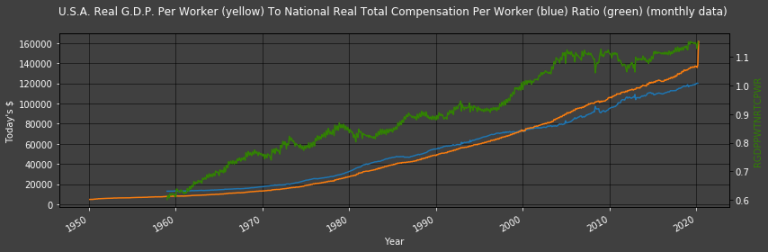
The graph above displays GDP and Total Compensation per worker figures as well as the ratio between the two (the latter is shown in green). It is this ratio that we use as our 𝑟r in the estimation model:
Since (as per Appendix 1) we deffined 𝑟𝑡 = 𝑅𝐺𝐷𝑃𝑃𝑊𝑡 / 𝑅𝑁𝑇𝐶𝑃𝑊𝑡, 𝑟𝑡−1 values do not need to be forecasted or modeled - we have the data needed to compute 𝑟𝑡−1 = 𝑅𝐺𝐷𝑃𝑃𝑊𝑡 − 1 / 𝑅𝑁𝑇𝐶𝑃𝑊𝑡−1.
𝑟𝑡 values - however - require values of 𝑅𝐺𝐷𝑃𝑃𝑊𝑡 for month 𝑡t, which are not published: this is where an estimate of ˆrt comes in useful.
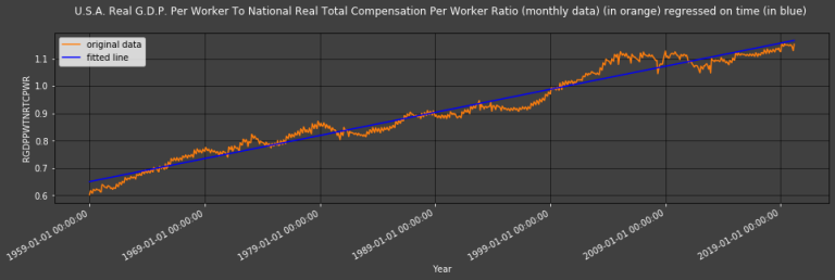
How may we model our estimate of 𝑟𝑡? The first models that come to mind are linear regression models; the below investigates the regression of USA Real GDP Per Worker To National Real Total Compensation Ratio (RGDPPWTNRTCPWR) against time (i.e.: months).
Regression of USA Real GDP Per Worker To National Real Total Compensation Per Worker Ratio against time
Here we use RGDPPWTNRTCPWR as 𝑟r such that 𝑦𝑡ˆ = 𝑐 + 𝛽𝑥𝑡 where 𝑦𝑡ˆ = 𝑅𝐺𝐷𝑃𝑃𝑊𝑇𝑁𝑅𝑇𝐶𝑃𝑊𝑅𝑡ˆ = 𝑟𝑡ˆ , 𝑥𝑡 is time in months, and 𝑐 & 𝛽 are computed to reduce the error of this model (i.e.: to reduce the 'error' term - ϵ - in 𝑦𝑡 = 𝑐 + 𝛽𝑥𝑡 + 𝜖𝑡 where 𝑦𝑡 = 𝑅𝐺𝐷𝑃𝑃𝑊𝑇𝑁𝑅𝑇𝐶𝑃𝑊𝑅𝑡 = 𝑟𝑡) via Ordinary Least Square estimation:
# First: Fit the trend
x = numpy.array([numpy.float64(i) for i in range(0, len(df["RGDPPWTNRTCPWR (monthly data)"].dropna()))])
y = numpy.array([numpy.float64(i) for i in df["RGDPPWTNRTCPWR (monthly data)"].dropna()])
(slope, intercept, r_value, p_value, std_err) = (scipy.stats.linregress(x = x, y = y))
df["RGDPPWTNRTCPWR regressed on months"] = (intercept + slope * x) - (df["RGDPPWTNRTCPWR (monthly data)"].dropna() * 0)
df["RGDPPWTNRTCPWR regressed on months' errors"] = df["RGDPPWTNRTCPWR regressed on months"] - df["RGDPPWTNRTCPWR (monthly data)"].dropna()
# Second: Plot it:
Plot_Regression(title = "U.S.A. Real G.D.P. Per Worker To National Real Total Compensation Per Worker Ratio (monthly data) (in orange) regressed on time (in blue)",
x = x, y = y, slope = slope, intercept = intercept,
data_point_type = "-", ylabel = "RGDPPWTNRTCPWR",
time_index_step = 12*10, figuresize = (16,4),
time_index = df["RGDPPWTNRTCPWR (monthly data)"].dropna().index)
# Third: Evaluate it:
Statistics_Table(dataset1 = df).loc[["RGDPPWTNRTCPWR (monthly data)",
"RGDPPWTNRTCPWR regressed on months",
"RGDPPWTNRTCPWR regressed on months' errors"],
["Mean of Absolute Values"]]

| Mean of Absolute Values | |
| RGDPPWTNRTCPWR (monthly data) | 0.907876 |
| RGDPPWTNRTCPWR regressed on months | 0.907876 |
| RGDPPWTNRTCPWR regressed on months' errors | 0.0241528 |
The statistics table shows a healthily low absolute (as in: ignoring the sign) error mean value for RGDPPWTNRTCPWR's regression model of 0.0242910.024291.
We seem to have gathered evidence that a time-linear model may be a good way to estimate 𝑟r and then monthly GDP. Remember that we will measure the effectiveness of our models by how they estimate GDP values at lower frequencies than they are published by official bodies (here: monthly, using monthly released Total Compensation data); an accurate estimation of our ratio is therefore paramount. One may thus attempt to look at estimates produced by methods other than straight forward linear regressions, e.g.: the Holt-Winters method. Let's investigate that method too:
Holt-Winters method
All estimation methods are to be used recursively. The Holt-Winters method makes sure that forecasts are heavily influenced by latest values by design. It offers better (i.e.: lower) model error (see model fit graph below) than our linear regressions too.
Nota Bene (N.B.): A non multiplicative Holt-Winters method is used here as computational limits mean that multiplicative Holt-Winters methods result in very many 'NaN' estimates that are unusable.
The cell below creates recursive RGDPPWTNRTCPWR Holt-Winters exponential smoothing estimates (RGDPPWTNRTCPWRHW); this means that we are using 𝑅𝐺𝐷𝑃𝑃𝑊𝑇𝑁𝑅𝑇𝐶𝑃𝑊𝑅𝑡−1 as 𝑟𝑡−1 and 𝑅𝐺𝐷𝑃𝑃𝑊𝑇𝑁𝑅𝑇𝐶𝑃𝑊𝑅𝐻𝑊𝑡 as 𝑟𝑡ˆ :
# The following for loop will throw errors informing us that the unspecified Holt-Winters Exponential Smoother
# parameters will be chosen by the default ' statsmodels.tsa.api.ExponentialSmoothing ' optimal ones.
# This is preferable and doesn't need to be stated for each iteration in the loop.
warnings.simplefilter("ignore")
RGDPPWTNRTCPWRHW_model_fit = statsmodels.tsa.api.ExponentialSmoothing(df["RGDPPWTNRTCPWR (monthly data)"].dropna(),
seasonal_periods = 12,
trend = 'add',
damped=True).fit(use_boxcox=True)
df["RGDPPWTNRTCPWRHW fitted values (monthly data)"] = RGDPPWTNRTCPWRHW_model_fit.fittedvalues
df["RGDPPWTNRTCPWRHW forecasts (monthly data)"] = RGDPPWTNRTCPWRHW_model_fit.forecast(12*4)
df["RGDPPWTNRTCPWRHW fitted values' real errors (monthly data)"] = df["RGDPPWTNRTCPWRHW fitted values (monthly data)"] - df["RGDPPWTNRTCPWR (monthly data)"]
# See the HW model's forecasts:
RGDPPWTNRTCPWRHW_model_fit.forecast(12)
| 01/04/2020 | 1.143114 |
| 01/05/2020 | 1.143141 |
| 01/06/2020 | 1.143158 |
| 01/07/2020 | 1.143169 |
| 01/08/2020 | 1.143176 |
| 01/09/2020 | 1.14318 |
| 01/10/2020 | 1.143183 |
| 01/11/2020 | 1.143185 |
| 01/12/2020 | 1.143186 |
| 01/01/2021 | 1.143186 |
| 01/02/2021 | 1.143187 |
| 01/03/2021 | 1.143187 |
Freq: MS, dtype: float64
# Plot the newly created Exponential Smoothing data
fig1, ax1 = plt.subplots(figsize=(12,4), facecolor="0.25")
df["RGDPPWTNRTCPWR (monthly data)"].dropna().plot(style = '-',
color = "blue",
legend = True).legend(["RGDPPWTNRTCPWR (monthly data)"])
RGDPPWTNRTCPWRHW_model_fit.fittedvalues.plot(style = '-',
color = "C1",
label = "RGDPPWTNRTCPWRHW model fit",
legend = True)
RGDPPWTNRTCPWRHW_model_fit.forecast(12).plot(style = '-',
color = "#328203",
label = "RGDPPWTNRTCPWRHW model forecast",
legend = True)
ax1.set_facecolor("0.25")
ax1.tick_params(axis = "both", colors = "w")
plt.ylabel("Ratio", color = "w")
ax1.set_xlabel("Years", color = "w")
ax1.grid(color = "black", linewidth = 0.5)
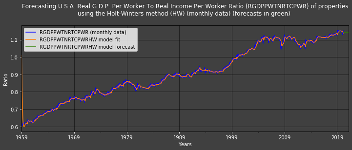
ax1.set_title("Forecasting U.S.A. Real G.D.P. Per Worker To Real Income Per Worker Ratio (RGDPPWTNRTCPWR) of properties" +
"\nusing the Holt-Winters method (HW) (monthly data) (forecasts in green)" +
" \n", color='w')
ax1.legend()
plt.show()
warnings.simplefilter("default") # We want our program to let us know of warnings from now on; they were only disabled for the for loop above.
Statistics_Table(dataset1 = df).loc[["RGDPPWTNRTCPWR regressed on months' errors",
"RGDPPWTNRTCPWRHW fitted values' real errors (monthly data)"],
["Mean of Absolute Values"]]

| Mean of Absolute Values | |
| RGDPPWTNRTCPWR regressed on months' errors | 0.0241528 |
| RGDPPWTNRTCPWRHW fitted values' real errors (monthly data) | 0.00773767 |
The Holt-Winters model's estimates - 𝑟ˆr^ - (in yellow) closely follow the realised RGDPPWTNRTCPWR values. This only holds untrue at the start (approximately for the first 2 years) when the model needs training. The (short) green line shows monthly forecasts for the next 4 years computed with this Holt-Winters model.
The statistics table clearly hows that the Holt -Winters model performs much better than the time-linear regression model: its errors are - on average - a lot lower (i.e: 0.0077352<0.024291).
Backtesting our Method
The Python function defined in the cell below returns the In-Sample Recursive Prediction values of ' data ' using the Holt-Winters exponential smoother Plus it then provides forecasts for One Out-Of-Sample period (thus the acronym 'ISRPHWPOOOF'):
def ISRPHWPOOOF(data_set, dataset_name, start, result_name, enforce_cap = False, cap = 1.1):
""" This is a function created specifically for this article/study. returns the In-Sample Recursive
Prediction values of ' data ' using the Holt-Winters exponential smoother Plus it then provides
forecasts for One Out-Of-Sample period (thus the acronym 'ISRPHWPOOOF').
data_set (pandas dataframe): Pandas data-frame where the data is stored
dataset_name (str): Our data is likely to be in a pandas dataframe with dates
for indexes in order to alleviate any date sinking issues. As a result, this
line allows the user to specify the column within such a dataset to use.
start (str): The start of our in-sample recursive prediction window. This value can be changed.
result_name (str): name given to the result column.
enforce_cap (bool): Set to False by default. The H-W model sometimes returns extremely large
values that do not fit in our set. This is a convergence issue. Applying an arbitrary cap allows
us to account for this.
cap (int/float): Set to ' 1.1 ' by default. This is the cap applied to the returned values if
' enforce_cap ' is set to True.
"""
# The following for loop will throw errors informing us that the unspecified Holt-Winters
# Exponential Smoother parameters will be chosen by the default
# ' statsmodels.tsa.api.ExponentialSmoothing ' optimal ones.
# This is preferable and doesn't need to be stated for each iteration in the loop.
warnings.simplefilter("ignore")
# We create an empty list (to get appended/populated)
# for our dataset's forecast using the Holt-Winters exponential smoother.
data_model_in_sample_plus_one_forecast = []
# Empty lists to be populated by our forecasts (in- or out-of-sample)
value, index = [], []
# the ' len(...) ' function here returns the number of rows in our dataset from our starting date till its end.
for i in range(0,len(data_set[dataset_name].loc[pandas.Timestamp(start):].dropna())):
# This line defines ' start_plus_i ' as our starting date plus i months
start_plus_i = str(datetime.datetime.strptime(start, "%Y-%m-%d") + dateutil.relativedelta.relativedelta(months=+i))[:10]
HWESi = statsmodels.tsa.api.ExponentialSmoothing(data_set[dataset_name].dropna().loc[:pandas.Timestamp(start_plus_i)],
trend = 'add', seasonal_periods = 12,
damped = True).fit(use_boxcox = True).forecast(1)
# This(following) outputs a forecast for one period ahead (whether in-sample or out of sample).
# Since we start at i = 0, this line provides a HW forecast for i at 1; similarly, at the
# last i (say T), it provides the first and only out-of-sample forecast (where i = T+1).
data_model_in_sample_plus_one_forecast.append(HWESi)
try:
if enforce_cap == True:
if float(str(HWESi)[14:-25]) > cap:
value.append(float(str(HWESi)[14:-25]))
else:
value.append(numpy.nan) # If the ratio
else:
value.append(float(str(HWESi)[14:-25]))
except:
# This adds NaN (Not a Number) to the list ' values ' if there is no value to add.
# The statsmodels.tsa.api.ExponentialSmoothing function sometimes (rarely) outputs NaNs.
value.append(numpy.nan)
finally:
# This adds our indecies (dates) to the list ' index '
index.append(str(HWESi)[:10])
# We want our program to let us know of warnings from now on; they were only disabled for the for loop above.
warnings.simplefilter("default")
return pandas.DataFrame(data = value, index = index, columns = [result_name])
We will back-test our models from January 1990
start = "1990-01-01"
df["RGDPPWTNRTCPWRHW fitted values' real errors from " + str(start) + " (monthly data)"] = df["RGDPPWTNRTCPWRHW fitted values (monthly data)"].loc[start:] - df["RGDPPWTNRTCPWR (monthly data)"].loc[start:]
# Model:
RGDPPWTNRTCPWRHW_model_in_sample_plus_one_forecast = ISRPHWPOOOF(data_set = df,
dataset_name = "RGDPPWTNRTCPWR (monthly data)",
start = start,
result_name = "RGDPPWTNRTCPWRHW model in sample plus one forecast")
df = pandas.merge(df, RGDPPWTNRTCPWRHW_model_in_sample_plus_one_forecast,
how = "outer", left_index = True, right_index = True)
# Model's errors:
RGDPPWTNRTCPWRHW_model_in_sample_plus_one_forecast_error = pandas.DataFrame(df["RGDPPWTNRTCPWR (monthly data)"] - df["RGDPPWTNRTCPWRHW model in sample plus one forecast"],
columns = ["RGDPPWTNRTCPWRHW model in sample plus one forecast error"])
df = pandas.merge(df, RGDPPWTNRTCPWRHW_model_in_sample_plus_one_forecast_error.dropna(),
how = "outer", left_index = True, right_index = True)
Remember that the ratio 𝑟𝑡rt is𝑅𝐺𝐷𝑃𝑃𝑊𝑡 / 𝑅𝑁𝑇𝐶𝑃𝑊𝑡RGDPPWtRNTCPWt, but 'today' (i.e.: at time 𝑡t), there is no 𝑅𝐺𝐷𝑃𝑃𝑊𝑡 value we can use (since only quarterly figures are published), this is why we made a forecast. As a result, we will differentiate between 𝑟𝑡ˆ as including the forecast (actually used as an estimate) at time 𝑡t as ' r_f ' ('f' for forecasted) and 𝑟𝑡−1 as ' r ' which does not use forecasts:
r = df["RGDPPWTNRTCPWR (monthly data)"].dropna()
r_f = df["RGDPPWTNRTCPWRHW model in sample plus one forecast"].dropna()
df["r"] = r
df["r_f"] = r_f
Plot1ax(df, datasubset = [-1,-2], datarange = ["1990-01-01",-1], ylabel = "Ratio",
title = "Real G.D.P. Per Worker To National Real Total Compensation Per Worker Ratio realised (r) and\nmodeled estimates using forecasts (r_f) starting on Jan. 1990",)
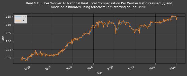

Modeled estimates (r_f) follow the realised 𝑟r values (r) so closely that it is difficult to differentiate them.
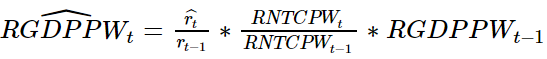
Remember also that 𝑅𝐺𝐷𝑃𝑃𝑊𝑡 = ( 𝑟𝑡 / 𝑟𝑡−1 )∗ ( 𝑅𝑁𝑇𝐶𝑃𝑊𝑡 / 𝑅𝑁𝑇𝐶𝑃𝑊𝑡−1 ) ∗ 𝑅𝐺𝐷𝑃𝑃𝑊𝑡−1, thus: RGDPPW estimate = 𝑅𝐺𝐷𝑃𝑃𝑊𝑡ˆ = (𝑟𝑡ˆ / 𝑟𝑡ˆ−1 ) ∗ ( 𝑅𝑁𝑇𝐶𝑃𝑊𝑡 / 𝑅𝑁𝑇𝐶𝑃𝑊𝑡−1 ) ∗ 𝑅𝐺𝐷𝑃𝑃𝑊𝑡−1
RGDPPW_estimate = (r_f / r.shift(1)) * (df["NRTCPW (monthly data)"] / df["NRTCPW (monthly data)"].shift(1)) * df["RGDPPW (monthly data)"].shift(1)
df["RGDPPW estimates"] = RGDPPW_estimate.dropna()
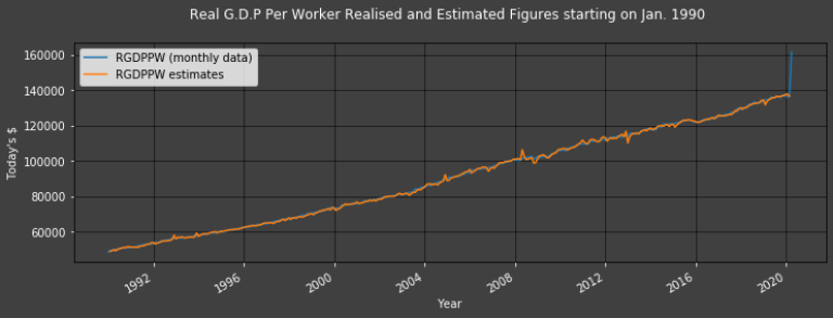
Yet again, looking at the realiations and model outputs on the same graph(s), it is difficult to see the model outputs because they follow realisations so well; the errors' graph and table shines a light on how small the error is:
Plot1ax(df, datasubset = [12,-1], datarange = ["1990-01-01",-1], ylabel = "Today's $", title = "Real G.D.P Per Worker Realised and Estimated Figures starting on Jan. 1990")
df["RGDPPW estimates' errors"] = df["RGDPPW (monthly data)"] - df["RGDPPW estimates"]
df["RGDPPW estimates' proportional errors"] = df["RGDPPW estimates' errors"] / df["RGDPPW (monthly data)"]
Plot2ax(dataset = df, leftaxisdata = [-2], rightaxisdata = [-1], title = "Real G.D.P Per Worker Estimates' Real (blue) and Proportional (orange) Errors",
y1label = "RGDPPW estimates' real errors", y2label = "RGDPPW estimates' proportional errors", leftcolors = "w")


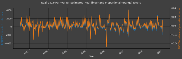
The difference between the lowest and 2nd lowest (as well as the highest and 2nd highest) troughs (and peaks) is less significant in the Proportional Error graph than in the straight forward Error graph.
Since RGDP figures are only released quarterly, it is best to investigate errors at each quarter
df["RGDPPW estimates' errors every quarter"] = df["RGDP (quarterly data)"] - df["RGDPPW estimates"]
Statistics_Table(dataset1 = df).loc[["RGDPPW estimates' errors", "RGDPPW estimates' proportional errors"],["Mean of Absolute Values"]]
| Mean of Absolute Values | |
| RGDPPW estimates' errors | 592.39 |
| RGDPPW estimates' proportional errors | 0.00666185 |
then:

df["RGDP estimates"] = df["RGDPPW estimates"] * df["USAWP (monthly data)"]
df[["RGDP (monthly data)", "RGDP estimates"]].dropna()
| RGDP (monthly data) | RGDP estimates | |
| 01/02/1990 | 5.87E+12 | 5.81E+12 |
| 01/03/1990 | 5.87E+12 | 5.86E+12 |
| 01/04/1990 | 5.87E+12 | 5.91E+12 |
| 01/05/1990 | 5.96E+12 | 5.85E+12 |
| 01/06/1990 | 5.96E+12 | 5.93E+12 |
| ... | ... | ... |
| 01/11/2019 | 2.17E+13 | 2.17E+13 |
| 01/12/2019 | 2.17E+13 | 2.17E+13 |
| 01/01/2020 | 2.17E+13 | 2.19E+13 |
| 01/02/2020 | 2.15E+13 | 2.19E+13 |
| 01/03/2020 | 2.15E+13 | 2.13E+13 |
It would be redundant testing the validity of these figures since we already did so when investigating Real GDP Per Worker estimates above.
Note also that for values today - at time 𝑇 - and/or close to today (e.g.: next month), 𝑅𝐺𝐷𝑃≈𝐺𝐷𝑃, and population growth is negligable, such that 𝑈𝑆𝐴𝑊𝑃𝑇 ≈ 𝑈𝑆𝐴𝑊𝑃𝑇+1, then:

It is therefore possible to use our method to predict future GDP values on a monthly basis.
References
You can find more detail regarding the DSWS API and related technologies for this article from the following resources:
- DSWS page on the Refinitiv Developer Community web site.
- DSWS API Quick Start Guide page.
- DSWS Tutorial page.
- DSWS API Python Reference Guide.
For any question related to this example or Eikon Data API, please use the Developers Community Q&A Forum.
Literature:
DOWNLOADS
Article.DataStream.Python.EstimatingMonthlyGDPFiguresViaAnIncomeApproachGitHub