
Gross Domestic Product (GDP) is often thought of and calculated with an Expenditure Approach such that
𝐺𝐷𝑃=𝐶+𝐼+𝐺+(𝑋−𝑀)
where 𝐶 = Consumption, 𝐼 = Investment, 𝐺 = Government Spending, & (𝑋–𝑀) = Net Exports.
The United States of America( USA)'s GDP (US GDP) is released quarterly by the Bureau of Economic Analysis, U.S. Department of Commerce. The only aforementioned component of US GDP released on a monthly basis is C, USA's Consumption Data. Monthly figures of GDP figures are thus not available, and estimating such values have proven of interest in academia (Mitchell, Smith, Weale, Wright, and Salazar (2005)) and in practice.
In this article, we will attempt to compute monthly US GDP estimates via the Holt-Winters (HW) method (resources on the HW model can be found here and - for academics - here). We then put ourselves in the shoes of an analyst who only has quarterly GDP component data (C, I, G or (X-M)). She/He uses the latest quarterly releases of GDP component datawhich spans from 2007 (in this study) to last quarter (last month at the earliest). She/He then uses the Holt-Winters method model to compute a forecast for the current period (month).
Accurate monthly GDP figures can be of great use in macroeconomic models going forward.
Development Tools & Resources
The example code demonstrating the use case is based on the following development tools and resources:
- Refinitiv's DataStream Web Services (DSWS): Access to DataStream data. A DataStream or Refinitiv Workspace IDentification (ID) will be needed to run the code bellow.
- Python Environment: Tested with Python 3.7
- Packages: DatastreamDSWS, Numpy, Pandas, statsmodel, scipy and Matplotlib. The Python built in modules warnings, statistics, datetime and dateutil are also required.
Tutorial Video Part 1 - Introduction to the Theory, Codebook and Python Libraries
Import libraries
# The ' from ... import ' structure here allows us to only import the
# module ' python_version ' from the library ' platform ':
from platform import python_version
print("This code runs on Python version " + python_version() + "\n")
This code runs on Python version 3.7.4
We need to gather our data. Since Refinitiv's DataStream Web Services (DSWS) allows for access to the most accurate and wholesome end-of-day (EOD) economic database (DB), naturally it is more than appropriate. We can access DSWS via the Python library "DatastreamDSWS" that can be installed simply by using pip install.
import DatastreamDSWS as DSWS
# We can use our Refinitiv's Datastream Web Socket (DSWS) API keys that allows us to be identified by Refinitiv's back-end services and enables us to request (and fetch) data:
# The username and password is placed in a text file so that it may be used in this code without showing it itself.
DSWS_username = open("Datastream_username.txt","r")
DSWS_password = open("Datastream_password.txt","r")
ds = DSWS.Datastream(username = str(DSWS_username.read()), password = str(DSWS_password.read()))
# It is best to close the files we opened in order to make sure that we don't stop any other services/programs from accessing them if they need to.
DSWS_username.close()
DSWS_password.close()
We use Refinitiv's Eikon Python Application Programming Interface (API) to access financial data. We can access it via the Python library "eikon" that can be installed simply by using pip install.
import eikon as ek
# The key is placed in a text file so that it may be used in this code without showing it itself:
eikon_key = open("eikon.txt","r")
ek.set_app_key(str(eikon_key.read()))
# It is best to close the files we opened in order to make sure that we don't stop any other services/programs from accessing them if they need to:
eikon_key.close()
The following are Python-built-in module/library, therefore it does not have a specific version number.
import os # os is a library used to manipulate files on machines
import datetime # datetime will allow us to manipulate Western World dates
import dateutil # dateutil will allow us to manipulate dates in equations
import warnings # warnings will allow us to manupulate warning messages (such as depretiation messages)
statistics, numpy, scipy and statsmodels are needed for datasets' statistical and mathematical manipulations
import statistics # This is a Python-built-in module/library, therefore it does not have a specific version number.
import numpy
import statsmodels
from statsmodels.tsa.api import ExponentialSmoothing, SimpleExpSmoothing, Holt
import scipy
from scipy import stats
for i,j in zip(["numpy", "statsmodels", "scipy"], [numpy, statsmodels, scipy]):
print("The " + str(i) + " library imported in this code is version: " + j.__version__)
The numpy library imported in this code is version: 1.16.5
The statsmodels library imported in this code is version: 0.10.1
The scipy library imported in this code is version: 1.3.1
pandas will be needed to manipulate data sets
import pandas
pandas.set_option('display.max_columns', None) # This line will ensure that all columns of our dataframes are always shown
print("The pandas library imported in this code is version: " + pandas.__version__)
The pandas library imported in this code is version: 0.25.1
matplotlib is needed to plot graphs of all kinds
import matplotlib
import matplotlib.pyplot as plt
print("The matplotlib library imported in this code is version: "+ matplotlib.__version__)
The matplotlib library imported in this code is version: 3.1.1
Setup Original Functions
Tutorial Video Part 2 - Introduction to Some Python Fundamentals and Our First Set of Functions
Setup data sets
The cell below defines a function that translates DataStream data into a shape we can work with: a Pandas Dafaframe normalised to the 1st of the month that it was collected in.
# This function will put Refinitiv's DataStream data into a Pandas Dafaframe and normalise it to the 1st of the month it was collected in.
def Translate_to_First_of_the_Month(data, dataname):
# The first 8 characters of the index is the ' yyyy-mm- ', onto which will be added '01'.
data.index = data.index.astype("str").str.slice_replace(8, repl = "01")
# This line resets the index to a pandas datetime format
data.index = pandas.to_datetime(data.index)
# This line renames the column as specified in the function
data.columns = [dataname]
return data
The cell below defines a function that appends our monthly data-frame with chosen data
df = pandas.DataFrame([])
def Add_to_df(data, dataname):
# The ' global df ' allows the function to take the pre-deffined variable ' df ' for granted and work from there
global df
DS_Data_monthly = Translate_to_First_of_the_Month(data, dataname)
# Note that the bellow is (purposefully) different to ' df[dataname] = DS_Data_monthly'
df = pandas.merge(df, DS_Data_monthly,
how = "outer",
left_index = True,
right_index=True)
pandas.plotting.register_matplotlib_converters() # Using an implicitly registered datetime converter for a matplotlib plotting method is no longer supported by matplotlib. Current versions of pandas requires explicitly registering matplotlib converters.
def Plot1ax(dataset, ylabel = "", title = "", xlabel = "Year",
datasubset = [0], datarange = False,
linescolor = False, figuresize = (12,4),
facecolor = "0.25", grid = True):
""" Plot1ax Version 2.0:
This function returns a Matplotlib graph with default colours and dimentions
on one y axis (on the left as oppose to two, one on the left and one on the right).
datasubset (list): Needs to be a list of the number of each column within
the dtaset that needs to be labled on the left.
datarange (bool): If wanting to plot graph from and to a specific point,
make datarange a list of start and end date.
linescolor (bool/list): (Default: False) This needs to be a list of the color of each
vector to be ploted, in order they are shown in their dataframe from left to right.
figuresize (tuple): (Default: (12,4)) This can be changed to give graphs of different
proportions. It is defaulted to a 12 by 4 (ratioed) graph.
facecolor (str): (Default: "0.25") This allows the user to change the
background color as needed.
grid (bool): (Default: "True") This allows us to decide wether or
not to include a grid in our pharphs.
"""
# This function works if the dataset is specified in names of columns
# or their placement (first column being the '0th').
if type(datasubset[0]) == int:
if datarange == False:
start_date = str(dataset.iloc[:,datasubset].index[0])
end_date = str(dataset.iloc[:,datasubset].index[-1])
else:
start_date = str(datarange[0])
if datarange[-1] == -1:
end_date = str(dataset.iloc[:,datasubset].index[-1])
else:
end_date = str(datarange[-1])
else:
if datarange == False:
start_date = str(dataset[datasubset].index[0])
end_date = str(dataset[datasubset].index[-1])
else:
start_date = str(datarange[0])
if datarange[-1] == -1:
end_date = str(dataset[datasubset].index[-1])
else:
end_date = str(datarange[-1])
fig, ax1 = plt.subplots(figsize = figuresize, facecolor = facecolor)
ax1.tick_params(axis = 'both', colors = 'w')
ax1.set_facecolor(facecolor)
fig.autofmt_xdate()
plt.ylabel(ylabel, color = 'w')
ax1.set_xlabel(str(xlabel), color = 'w')
if type(datasubset[0]) == int:
if linescolor == False:
for i in datasubset: # This is to label all the lines in order to allow matplot lib to create a legend
ax1.plot(dataset.iloc[:, i].loc[start_date : end_date],
label = str(dataset.columns[i]))
else:
for i in datasubset: # This is to label all the lines in order to allow matplot lib to create a legend
ax1.plot(dataset.iloc[:, i].loc[start_date : end_date],
label = str(dataset.columns[i]),
color = linescolor)
else:
if linescolor == False:
for i in datasubset: # This is to label all the lines in order to allow matplot lib to create a legend
ax1.plot(dataset[i].loc[start_date : end_date],
label = i)
else:
for i in datasubset: # This is to label all the lines in order to allow matplot lib to create a legend
ax1.plot(dataset[i].loc[start_date : end_date],
label = i,
color = linescolor)
ax1.tick_params(axis = 'y')
if grid == True:
ax1.grid(color='black', linewidth = 0.5)
ax1.set_title(str(title) + " \n", color = 'w')
plt.legend()
plt.show()
The cell below defines a function to plot data on two y axis.
def Plot2ax(dataset, rightaxisdata, y1label, y2label, leftaxisdata,
title = "", xlabel = "Year", y2color = "C1", y1labelcolor = "C0",
figuresize = (12,4), leftcolors = ('C1'), facecolor = "0.25"):
""" Plot2ax Version 2.0:
This function returns a Matplotlib graph with default colours and dimentions
on two y axis (one on the left and one on the right)
leftaxisdata (list): Needs to be a list of the number of each column within
the dtaset that needs to be labled on the left
figuresize (tuple): (Default: (12,4)) This can be changed to give graphs of
different proportions. It is defaulted to a 12 by 4 (ratioed) graph
leftcolors (str / tuple of (a) list(s)): This sets up the line color for data
expressed with the left hand y-axis. If there is more than one line,
the list needs to be specified with each line colour specified in a tuple.
facecolor (str): (Default: "0.25") This allows the user to change the
background color as needed
"""
fig, ax1 = plt.subplots(figsize = figuresize, facecolor = facecolor)
ax1.tick_params(axis = 'both', colors = 'w')
ax1.set_facecolor(facecolor)
fig.autofmt_xdate()
plt.ylabel(y1label, color = y1labelcolor)
ax1.set_xlabel(str(xlabel), color = 'w')
ax1.set_ylabel(str(y1label))
for i in leftaxisdata: # This is to label all the lines in order to allow matplot lib to create a legend
ax1.plot(dataset.iloc[:, i])
ax1.tick_params(axis = 'y')
ax1.grid(color='black', linewidth = 0.5)
ax2 = ax1.twinx() # instantiate a second axes that shares the same x-axis
color = str(y2color)
ax2.set_ylabel(str(y2label), color=color) # we already handled the x-label with ax1
plt.plot(dataset.iloc[:, list(rightaxisdata)], color=color)
ax2.tick_params(axis='y', labelcolor='w')
ax1.set_title(str(title) + " \n", color='w')
fig.tight_layout() # otherwise the right y-label is slightly clipped
plt.show()
The cell below defines a function to plot data regressed on time.
def Plot_Regression(x, y, slope, intercept, ylabel,
title = "", xlabel = "Year", facecolor = "0.25", data_point_type = ".", original_data_color = "C1",
time_index = [], time_index_step = 48,
figuresize = (12,4),
line_of_best_fit_color = "b"):
""" Plot_Regression Version 1.0:
Plots the regression line with its data with appropriate defult Refinitiv colours.
facecolor (str): (Default: "0.25") This allows the user to change the background color as needed
figuresize (tuple): (Default: (12,4)) This can be changed to give graphs of different proportions. It is defaulted to a 12 by 4 (ratioed) graph
line_of_best_fit_color (str): This allows the user to change the background color as needed.
' time_index ' and ' time_index_step ' allow us to dictate the fequency of the ticks on the x-axis of our graph.
"""
fig, ax1 = plt.subplots(figsize = figuresize, facecolor = facecolor)
ax1.tick_params(axis = "both", colors = "w")
ax1.set_facecolor(facecolor)
fig.autofmt_xdate()
plt.ylabel(ylabel, color = 'w')
ax1.set_xlabel(xlabel, color = 'w')
ax1.plot(x, y, data_point_type, label='original data', color = original_data_color)
ax1.plot(x, intercept + slope * x, 'r', label = 'fitted line', color = line_of_best_fit_color)
ax1.tick_params(axis = 'y')
ax1.grid(color='black', linewidth = 0.5)
ax1.set_title(title + " \n", color='w')
plt.legend()
if len(time_index) != 0:
# locs, labels = plt.xticks()
plt.xticks(numpy.arange(len(y), step = time_index_step),
[i for i in time_index[0::time_index_step]])
plt.show()
Setup Statistics Tools
def Single_period_Geometric_Growth(data):
data = list(data)
single_period_geometric_growth = ( (data[-1]/data[0])**(1/((len(data))-1)) ) - 1 # note that we use ' len(data) - 1 ' instead of ' len(data) ' as the former already lost its degree of freedom just like we want it to.
return single_period_geometric_growth
The cell below defines a function that creates and displays a table of statistics for all vectors (columns) within any two specified datasets.
def Statistics_Table(dataset1, dataset2 = ""):
Statistics_Table_Columns = list(dataset1.columns)
if str(dataset2) != "":
[Statistics_Table_Columns.append(str(i)) for i in dataset2.columns]
Statistics_Table = pandas.DataFrame(columns = ["Mean", "Mean of Absolute Values",
"Standard Deviation",
"Median", "Skewness",
"Kurtosis",
"Single Period Growth Geometric Average"],
index = [c for c in Statistics_Table_Columns])
def Statistics_Table_function(data):
for c in data.columns:
Statistics_Table["Mean"][str(c)] = numpy.mean(data[str(c)].dropna())
Statistics_Table["Mean of Absolute Values"][str(c)] = numpy.mean(abs(data[str(c)].dropna()))
Statistics_Table["Standard Deviation"][str(c)] = numpy.std(data[str(c)].dropna())
Statistics_Table["Median"][str(c)] = numpy.median(data[str(c)].dropna())
Statistics_Table["Skewness"][str(c)] = scipy.stats.skew(data[str(c)].dropna())
Statistics_Table["Kurtosis"][str(c)] = scipy.stats.kurtosis(data[str(c)].dropna())
if len(data[str(c)].dropna()) != 1 or data[str(c)].dropna()[0] != 0: # This if statement is needed in case we end up asking for the computation of a value divided by 0.
Statistics_Table["Single Period Growth Geometric Average"][str(c)] = Single_period_Geometric_Growth(data[str(c)].dropna())
Statistics_Table_function(dataset1)
if str(dataset2) != "":
Statistics_Table_function(dataset2)
return Statistics_Table
Monthly Data
U.S.A.'s Consumption Data
Add_to_df(data = ds.get_data(tickers = 'USPERCONB', # this is the ticker for United States, Personal Outlays, Personal Consumption Expenditure, Overall, Total, Current Prices, AR, SA, USD
fields = "X", # DataStream's default field is 'X'
start = '1950-02-01',
freq = 'M') * 1000000000, # This data is given in units of 1000000000
dataname = "Consumption (monthly data)")
Tutorial Video Part 3 - Collect Data and Our Second Set of Functions
Quarterly Data
# Our data is released quarterly, so we have to shape it into a monthly database. The function below will allow for this:
def Quarterly_To_Monthly(data, dataname, deflator = False):
"""Quarterly data can sometimes be recorded in a monthly data-frames.
This function returns a pandas data-frame in which inter-quarterly cells are populatd.
data (pandas.DataFrame): a pandas data-frame of the quarterly data
that is wanted in a monthly pandas data-frame
dataname (str): a string of the name wanted for the column of returned data-frame
deflator (bool): Set to False by default. If the data passed is an inflator,
setting ' deflator ' to True will inverse it)
"""
data_proper, data_full_index = [], []
for i in range(0, len(data)):
[data_proper.append(float(data.iloc[j])) for j in [i,i,i]]
[data_full_index.append(datetime.datetime.strptime(str(data.index[i])[0:8] + "01", "%Y-%m-%d") + dateutil.relativedelta.relativedelta(months =+ j)) for j in range(0,3)]
data = pandas.DataFrame(data = data_proper, columns = [dataname], index = data_full_index)
if deflator == True:
data = pandas.DataFrame(data = 1 / (data / data.iloc[-1]), columns = [dataname], index = data_full_index)
data.index = pandas.to_datetime(data.index)
return data
def Collect_Quarterly_Data(ticker, data_name, field = "X", start = "1950-02-01", freq = "M",
multiplier = 1):
""" This function was created specifically for this script/article. It decreases the
number of repeated code lines collecting data in several forms in our df.
ticker (str/list): string of the one DataStream ticker or list of multiple DataStream
tickers to be collected.
field (str): Set to "X" by default. Field to be collected fo rthe ticker(s) in question.
start (str): Set to "1950-02-01" by default. This is the date at which the data is to be
collected from on DataStream.
freq (str): Set to "M" by default. This is the frequency at which you would like the
data to be collected from DataStream. "M" for monthly, "Q" for quarterly, "A" for
annually, et cetera. If ' freq ' is set to a higher frequency than is available on
DataSream, the highest possible one will be used (exempli gratia: if asking for "M"
when only "Q" data is available, data will be collected as if freq = "Q").
multiplier (int/float): Set to ' 1 ' by default. Our collected data will be multiplied
by this multiplier.
"""
# Only DataStream requests returning numbers are meant to be ask for in this function.
# The following try loop will account for the case where DataStream returns something
# else (or somenthing else is asked of it):
try:
# The multiplier can only be used if data in ' dsdata ' is numeric
dsdata = ds.get_data(tickers = ticker, fields = field,
start = '1950-02-01', freq = 'M') * multiplier
except:
dsdata = ds.get_data(tickers = ticker, fields = field,
start = '1950-02-01', freq = 'M')
# Adding data for every quarter in our df:
Add_to_df(data = dsdata.copy(), dataname = data_name + " (quarterly data)")
# Adding quarterly data for every month in our df:
Add_to_df(data = Quarterly_To_Monthly(dsdata.copy(),
dataname = data_name + " (quarterly data)",
deflator = False),
dataname = data_name + " (monthly step data)")
Collect_Quarterly_Data(ticker = "USGFCF..B", data_name = "Investment", multiplier = 1000000000)
Collect_Quarterly_Data(ticker = "USCNGOV.B", data_name = "Government Investment", multiplier = 1000000000)
Collect_Quarterly_Data(ticker = "USBALGSVB", data_name = "Net Exports", multiplier = 1000000000)
Tutorial Video Part 4 - Dataframe manipulations and Plots
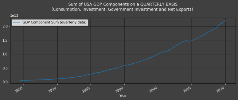
G.D.P. Component Sum
df["GDP Component Sum (quarterly data)"] = df.dropna()["Consumption (monthly data)"] + df.dropna()["Investment (quarterly data)"] + df.dropna()["Government Investment (quarterly data)"] + df.dropna()["Net Exports (quarterly data)"]
Plot1ax(dataset = pandas.DataFrame(df["GDP Component Sum (quarterly data)"].dropna()),
title = "Sum of USA GDP Components on a QUARTERLY BASIS\n(Consumption, Investment, Government Investment and Net Exports)")
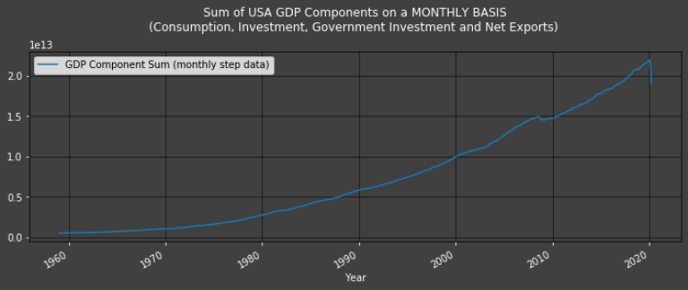
df["GDP Component Sum (monthly step data)"] = df["Consumption (monthly data)"] + df["Investment (monthly step data)"] + df["Government Investment (monthly step data)"] + df["Net Exports (monthly step data)"]
Plot1ax(dataset = pandas.DataFrame(df["GDP Component Sum (monthly step data)"].dropna()),
title = "Sum of USA GDP Components on a MONTHLY BASIS\n(Consumption, Investment, Government Investment and Net Exports)")
U.S.A.'s G.D.P.
To check our model, we can use 'United States, National Product Account, Gross Domestic Product, Overall, Total, Current Prices, AR, SA, USD'.
Add_to_df(data = ds.get_data(tickers = 'USGDP...B',
fields = "X",
start = '1950-02-01',
freq = 'M') * 1000000000,
dataname = "GDP (every quarter)")
df["GDP (monthly step data)"] = Quarterly_To_Monthly(data = df["GDP (every quarter)"],
dataname = "GDP (monthly step data)").dropna()
Data Résumé
Plot1ax(title = "USA GDP and its components (quarterly data)",
dataset = df.dropna(), ylabel = "Today's $",
datasubset = ["Investment (quarterly data)",
"Government Investment (quarterly data)",
"Net Exports (quarterly data)",
"Net Exports (quarterly data)",
"GDP Component Sum (quarterly data)",
"GDP (every quarter)"])
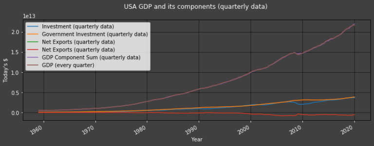
Note that the GDP and GDP Component Sum datapoints align so well that they are indistinguishable in the graph above
df
| Consumption (monthly data) | Investment (quarterly data) | Investment (monthly step data) | Government Investment (quarterly data) | Government Investment (monthly step data) | Net Exports (quarterly data) | Net Exports (monthly step data) | GDP Component Sum (quarterly data) | GDP Component Sum (monthly step data) | GDP (every quarter) | GDP (monthly step data) | |
| 01/02/1950 | NaN | 4.47E+10 | 4.47E+10 | 4.90E+10 | 4.90E+10 | 2.20E+09 | 2.20E+09 | NaN | NaN | 2.81E+11 | 2.81E+11 |
| 01/03/1950 | NaN | NaN | 4.47E+10 | NaN | 4.90E+10 | NaN | 2.20E+09 | NaN | NaN | NaN | 2.81E+11 |
| 01/04/1950 | NaN | NaN | 4.47E+10 | NaN | 4.90E+10 | NaN | 2.20E+09 | NaN | NaN | NaN | 2.81E+11 |
| 01/05/1950 | NaN | 4.95E+10 | 4.95E+10 | 4.96E+10 | 4.96E+10 | 1.64E+09 | 1.64E+09 | NaN | NaN | 2.90E+11 | 2.90E+11 |
| 01/06/1950 | NaN | NaN | 4.95E+10 | NaN | 4.96E+10 | NaN | 1.64E+09 | NaN | NaN | NaN | 2.90E+11 |
| ... | ... | ... | ... | ... | ... | ... | ... | ... | ... | ... | ... |
| 01/03/2020 | 1.39E+13 | NaN | 3.67E+12 | NaN | 3.85E+12 | NaN | -5.26E+11 | NaN | 2.09E+13 | NaN | 2.15E+13 |
| 01/04/2020 | 1.20E+13 | NaN | 3.67E+12 | NaN | 3.85E+12 | NaN | -5.26E+11 | NaN | 1.90E+13 | NaN | 2.15E+13 |
| 01/05/2020 | NaN | NaN | NaN | NaN | NaN | NaN | NaN | NaN | NaN | NaN | NaN |
| 01/06/2020 | NaN | NaN | NaN | NaN | NaN | NaN | NaN | NaN | NaN | NaN | NaN |
| 01/07/2020 | NaN | NaN | NaN | NaN | NaN | NaN | NaN | NaN | NaN | NaN | NaN |
Tutorial Video Part 5 - The Holt Winters Model for Positive Values
Tutorial Video Part 6 - The Holt Winters Model for Negative Values
def Hot_Winters_Method(name, forecast_period = 3, negative_accounting = False, silence_warings = True,
figure_size = (15,4), face_color = "0.25", point_style = "-", plot_color = "blue",
fitted_point_style = "-", fitted_point_color = "C1", xlabel = "Years",
forecasted_point_style = "-", forecasted_point_color = "#328203"):
""" This function was created specifically for this script/article. It uses the Holt-Winters
method to construct estimates and forecasts, adds it to ' df 'and plots the original data against
the estimates and forecasts.
Necessitates the function ' Quarterly_To_Monthly '
name (str): Name of the GDP component in question. This component must be included in ' df '.
forecast_period (int): Set to ' 3 ' as default. Number of periods we wish to display forecasts for.
negative_accounting (bool): Set to False by default. If set to True, this accounts for negative values
in that it does not display forecasted values explicitly or the graph because they would be shifted up.
figure_size, face_color, point_style, plot_color, fitted_point_style, fitted_point_color, xlabel,
forecasted_point_style, and forecasted_point_color are variables to modify the plot returned.
"""
global df
if negative_accounting == True:
# First: we need to note that the Holt-Winters model only works for positive datasets.
# the following is to account for negative values:
_data_min_p1 = numpy.absolute(pandas.DataFrame.min(df[name + " (monthly step data)"])) + 1
_data = (_data_min_p1 + df[name + " (monthly step data)"].copy()).dropna()
df[name + " (monthly step data) positive"] = _data
else:
_data_min_p1 = 0
_data = df[name + " (monthly step data)"].dropna()
if silence_warings == True:
# The following will throw errors informing us that the unspecified Holt-Winters Exponential Smoother
# parameters will be chosen by the default ' statsmodels.tsa.api.ExponentialSmoothing ' optimal ones.
# This is preferable and doesn't need to be stated for each iteration in the loop.
warnings.simplefilter("ignore")
model_fit = statsmodels.tsa.holtwinters.ExponentialSmoothing(_data.dropna(),
seasonal_periods = 12,
trend = 'add',
damped=True).fit(use_boxcox=True)
df[name + " fitted values (monthly step data)"] = model_fit.fittedvalues - _data_min_p1
df[name + " forecasts (monthly step data)"] = model_fit.forecast(forecast_period) - _data_min_p1
df[name + " fitted values' real errors (monthly step data)"] = df[name + " fitted values (monthly step data)"] - df[name + " (monthly step data)"]
if negative_accounting == False:
# See the HW model's forecasts:
print(name + " forecasts:")
display(model_fit.forecast(forecast_period))
# Plot the newly created Exponential Smoothing data
fig1, ax1 = plt.subplots(figsize = figure_size, facecolor = face_color)
df[name + " (monthly step data)"].dropna().plot(style = point_style,
color = plot_color,
legend = True).legend([name + " (monthly step data)"])
model_fit.fittedvalues.plot(style = fitted_point_style,
color = fitted_point_color,
label = name + " model fit",
legend = True)
model_fit.forecast(forecast_period).plot(style = forecasted_point_style,
color = forecasted_point_color,
label = name + " model forecast",
legend = True)
ax1.set_facecolor(face_color)
ax1.tick_params(axis = "both", colors = "w")
plt.ylabel("Ratio", color = "w")
ax1.set_xlabel(xlabel, color = "w")
ax1.grid(color='black', linewidth = 0.5)
# The default 'forecasted_point_color' is "#328203", i.e.: green
if forecasted_point_color == "#328203":
ax1.set_title("Forecasting USA Real GDP's "+ name + " component of properties" +
"\nusing the Holt-Winters method (HW) (monthly data) (forecasts in green)" +
" \n", color='w')
else:
ax1.set_title("Forecasting U.S.A. Real G.D.P.'s "+ name + " component of properties" +
"\nusing the Holt-Winters method (HW) (monthly data) (forecasts in " +
forecasted_point_color + ") \n", color='w')
ax1.legend()
plt.show()
if silence_warings == True:
# We want our program to let us know of warnings from now on; they were only disabled for the for loop above.
warnings.simplefilter("default")
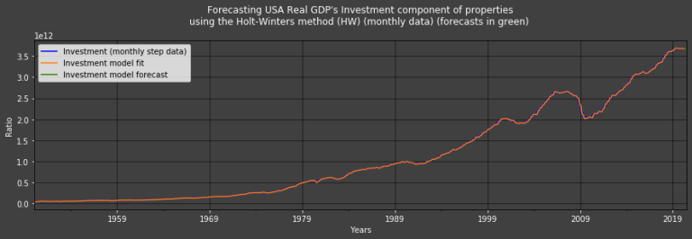
U.S.A.'s Investments' Estimates using the HW method
Hot_Winters_Method(name = "Investment")
Investment forecasts:
2020-05-01 3.666572e+12
2020-06-01 3.664588e+12
2020-07-01 3.662814e+12
Freq: MS, dtype: float64
# the ' pandas.DataFrame ' here is only there to make Jupyter return a Markdown table that looks better than the raw ' print ' output.
pandas.DataFrame(Statistics_Table(dataset1 = df).loc[["Investment forecasts (monthly step data)",
"Investment fitted values' real errors (monthly step data)"]]["Mean of Absolute Values"])
| Mean of Absolute Values | |
| Investment forecasts (monthly step data) | 3.66E+12 |
| Investment fitted values' real errors (monthly step data) | 7.88E+09 |
U.S.A.'s Government Investment using the HW method
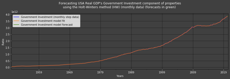
Hot_Winters_Method(name = "Government Investment")
Government Investment forecasts:
2020-05-01 3.866815e+12
2020-06-01 3.876213e+12
2020-07-01 3.885344e+12
Freq: MS, dtype: float64
U.S.A.'s Net Exports of Goods and Services using the HW method
Hot_Winters_Method(name = "Net Exports", negative_accounting = True)
df with Holt-Winters estimates
df
| Consumption (monthly data) | Investment (quarterly data) | Investment (monthly step data) | Government Investment (quarterly data) | Government Investment (monthly step data) | Net Exports (quarterly data) | Net Exports (monthly step data) | GDP Component Sum (quarterly data) | GDP Component Sum (monthly step data) | GDP (every quarter) | GDP (monthly step data) | Investment fitted values (monthly step data) | Investment forecasts (monthly step data) | Investment fitted values' real errors (monthly step data) | Government Investment fitted values (monthly step data) | Government Investment forecasts (monthly step data) | Government Investment fitted values' real errors (monthly step data) | Net Exports (monthly step data) positive | Net Exports fitted values (monthly step data) | Net Exports forecasts (monthly step data) | Net Exports fitted values' real errors (monthly step data) | |
| 01/02/1950 | NaN | 4.47E+10 | 4.47E+10 | 4.90E+10 | 4.90E+10 | 2.20E+09 | 2.20E+09 | NaN | NaN | 2.81E+11 | 2.81E+11 | 4.47E+10 | NaN | 1.53E-05 | 4.87E+10 | NaN | -2.13E+08 | 8.08E+11 | 2.20E+09 | NaN | 6.10E-04 |
| 01/03/1950 | NaN | NaN | 4.47E+10 | NaN | 4.90E+10 | NaN | 2.20E+09 | NaN | NaN | NaN | 2.81E+11 | 4.47E+10 | NaN | 1.53E-05 | 4.90E+10 | NaN | 7.02E+07 | 8.08E+11 | 2.20E+09 | NaN | 6.10E-04 |
| 01/04/1950 | NaN | NaN | 4.47E+10 | NaN | 4.90E+10 | NaN | 2.20E+09 | NaN | NaN | NaN | 2.81E+11 | 4.47E+10 | NaN | 1.53E-05 | 4.91E+10 | NaN | 1.92E+08 | 8.08E+11 | 2.20E+09 | NaN | 6.10E-04 |
| 01/05/1950 | NaN | 4.95E+10 | 4.95E+10 | 4.96E+10 | 4.96E+10 | 1.64E+09 | 1.64E+09 | NaN | NaN | 2.90E+11 | 2.90E+11 | 4.47E+10 | NaN | -4.73E+09 | 4.92E+10 | NaN | -4.68E+08 | 8.07E+11 | 2.20E+09 | NaN | 5.60E+08 |
| 01/06/1950 | NaN | NaN | 4.95E+10 | NaN | 4.96E+10 | NaN | 1.64E+09 | NaN | NaN | NaN | 2.90E+11 | 4.84E+10 | NaN | -1.10E+09 | 4.96E+10 | NaN | -3.65E+07 | 8.07E+11 | 1.68E+09 | NaN | 3.43E+07 |
| ... | ... | ... | ... | ... | ... | ... | ... | ... | ... | ... | ... | ... | ... | ... | ... | ... | ... | ... | ... | ... | ... |
| 01/03/2020 | 1.39E+13 | NaN | 3.67E+12 | NaN | 3.85E+12 | NaN | -5.26E+11 | NaN | 2.09E+13 | NaN | 2.15E+13 | 3.67E+12 | NaN | 3.05E+09 | 3.85E+12 | NaN | 2.84E+09 | 2.79E+11 | -5.25E+11 | NaN | 8.10E+08 |
| 01/04/2020 | 1.20E+13 | NaN | 3.67E+12 | NaN | 3.85E+12 | NaN | -5.26E+11 | NaN | 1.90E+13 | NaN | 2.15E+13 | 3.67E+12 | NaN | -1.43E+09 | 3.86E+12 | NaN | 1.34E+10 | 2.79E+11 | -5.18E+11 | NaN | 8.11E+09 |
| 01/05/2020 | NaN | NaN | NaN | NaN | NaN | NaN | NaN | NaN | NaN | NaN | NaN | NaN | 3.67E+12 | NaN | NaN | 3.87E+12 | NaN | NaN | NaN | -5.20E+11 | NaN |
| 01/06/2020 | NaN | NaN | NaN | NaN | NaN | NaN | NaN | NaN | NaN | NaN | NaN | NaN | 3.66E+12 | NaN | NaN | 3.88E+12 | NaN | NaN | NaN | -5.18E+11 | NaN |
| 01/07/2020 | NaN | NaN | NaN | NaN | NaN | NaN | NaN | NaN | NaN | NaN | NaN | NaN | 3.66E+12 | NaN | NaN | 3.89E+12 | NaN | NaN | NaN | -5.16E+11 | NaN |
Tutorial Video Part 7 - Backtesting our Method
The Setting for this video has changed, I do apologize for the lighting!
def ISRPHWPOOOF(data_set, dataset_name, start, result_name, enforce_cap = False, cap = 1.1):
""" ISRPHWPOOOF Version 3.0:
data_set (pandas dataset): dataframe where the data is stored
dataset_name (str): Our data is likely to be in a pandas dataframe with dates for
indexes in order to alleviate any date sinking issues. As a result, this line allows
the user to specify the column within such a dataset to use.
start (str): The start of our in-sample recursive prediction window. e.g.: "1990-01-01".
This value can be changed.
enforce_cap (bool): Set to False by default.
cap (int/float): Set to ' 1.1 ' by default.
"""
# The following for loop will throw errors informing us that the unspecified Holt-Winters
# Exponential Smoother parameters will be chosen by the default
# ' statsmodels.tsa.holtwinters.ExponentialSmoothing ' optimal ones. This is preferable and
# doesn't need to be stated for each iteration in the loop.
warnings.simplefilter("ignore")
# We create an empty list (toget appended/populated) for our dataset's forecast using the
# Holt-Winters exponential smoother and to be populated by our forecasts (in- or out-of-sample)
data_model_in_sample_plus_one_forecast, value, index = [], [], []
# the ' len(...) ' function here returns the number of rows in our dataset from our starting date till its end.
for i in range(0,len(data_set[dataset_name].loc[pandas.Timestamp(start):].dropna())):
# This line deffines ' start_plus_i ' as our starting date plus i months
start_plus_i = str(datetime.datetime.strptime(start, "%Y-%m-%d") + dateutil.relativedelta.relativedelta(months=+i))[:10]
HWESi = statsmodels.tsa.holtwinters.ExponentialSmoothing(data_set[dataset_name].dropna().loc[:pandas.Timestamp(start_plus_i)],
trend = 'add',
seasonal_periods = 12,
damped = True).fit(use_boxcox = True).forecast(1)
# This outputs a forecast for one period ahead (whether in-sample or out of sample). Since we start at i = 0, this line provides a HW forecast for i at 1;
# similarly, at the last i (say T), it provides the first and only out-of-sample forecast (where i = T+1).
data_model_in_sample_plus_one_forecast.append(HWESi)
try:
# Sometimes the H-W model comes up with extreme estimates, a cap can account for that:
if enforce_cap == True:
if float(str(HWESi)[14:-25]) > cap:
value.append(float(str(HWESi)[14:-25]))
else:
value.append(numpy.nan) # If the ratio
else:
value.append(float(str(HWESi)[14:-25]))
except:
# This adds NaN (Not a Number) to the list ' values ' if there is no value to add.
# The statsmodels.tsa.api.ExponentialSmoothing function sometimes (rarely) outputs NaNs.
value.append(numpy.nan)
finally:
# This adds our indecies (dates) to the list ' index '
index.append(str(HWESi)[:10])
# We want our program to let us know of warnings from now on; they were only disabled for the for loop above.
warnings.simplefilter("default")
return pandas.DataFrame(data = value, index = index, columns = [result_name])
We will back-test our models from January 1990
start = "2007-01-01"
Backtesting our Method with Investment data
# Model:
Investment_model_in_sample_plus_one_forecast = ISRPHWPOOOF(data_set = df,
dataset_name = "Investment (monthly step data)",
start = start,
result_name = "Investment model in sample plus one forecast")
df = pandas.merge(df, Investment_model_in_sample_plus_one_forecast,
how = "outer", left_index = True, right_index = True)
# Model's errors:
Investment_model_in_sample_plus_one_forecast_error = pandas.DataFrame(df["Investment (monthly step data)"] - df["Investment model in sample plus one forecast"],
columns = ["Investment model in sample plus one forecast error"])
df = pandas.merge(df, Investment_model_in_sample_plus_one_forecast_error.dropna(),
how = "outer", left_index = True, right_index = True)
Plot1ax(title = "Investment component of US GDP", datarange = [start,-1], ylabel = "Today's $",
dataset = df, datasubset = ["Investment (monthly step data)", "Investment model in sample plus one forecast"])
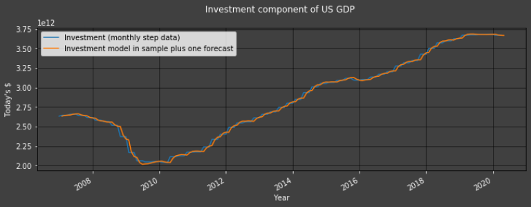
In the graph above, we put ourselves in the shoes of an analyst who only has quarterly Investment data. She/He uses the latest quarterly releases of Investment data which spans from 1950 (in our example) to last quarter (last month at the earliest). She/He then uses the HW model to compute a forecast for the current period (month) - in yellow in the graph above.
Backtesting our Method with Government Investment data
# Model:
Government_Investment_model_in_sample_plus_one_forecast = ISRPHWPOOOF(data_set = df,
dataset_name = "Government Investment (monthly step data)",
start = start,
result_name = "Government Investment model in sample plus one forecast")
df = pandas.merge(df, Government_Investment_model_in_sample_plus_one_forecast,
how = "outer", left_index = True, right_index = True)
# Model's errors:
Government_Investment_model_in_sample_plus_one_forecast_error = pandas.DataFrame(df["Government Investment (monthly step data)"] - df["Government Investment model in sample plus one forecast"],
columns = ["Government Investment model in sample plus one forecast error"])
df = pandas.merge(df, Government_Investment_model_in_sample_plus_one_forecast_error.dropna(),
how = "outer", left_index = True, right_index = True)
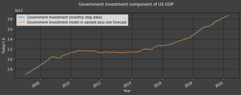
Plot1ax(title = "Government Investment component of US GDP", datarange = [start,-1], ylabel = "Today's $",
dataset = df, datasubset = ["Government Investment (monthly step data)",
"Government Investment model in sample plus one forecast"])
Backtesting our Method with Net Exports data
# Model:
Net_Exports_model_in_sample_plus_one_forecast = ISRPHWPOOOF(data_set = df,
dataset_name = "Net Exports (monthly step data) positive",
start = start,
result_name = "Net Exports model in sample plus one forecast")
Net_Exports_min_p1 = numpy.absolute(pandas.DataFrame.min(df["Net Exports (monthly step data)"])) + 1
df = pandas.merge(df, Net_Exports_model_in_sample_plus_one_forecast - Net_Exports_min_p1,
how = "outer", left_index = True, right_index = True)
# Model's errors:
Net_Exports_model_in_sample_plus_one_forecast_error = pandas.DataFrame(df["Net Exports (monthly step data)"] - df["Net Exports model in sample plus one forecast"],
columns = ["Net Exports model in sample plus one forecast error"])
df = pandas.merge(df, Net_Exports_model_in_sample_plus_one_forecast_error.dropna(),
how = "outer", left_index = True, right_index = True)
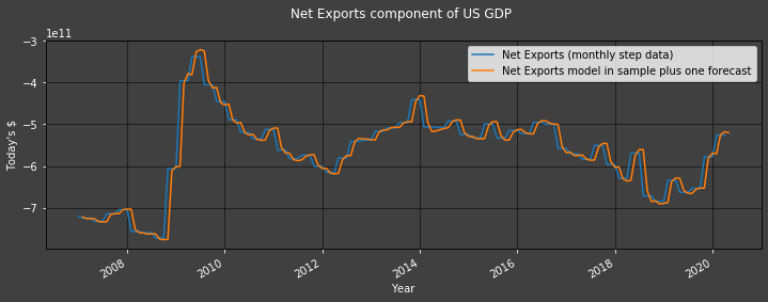
Plot1ax(title = "Net Exports component of US GDP", datarange = [start,-1], ylabel = "Today's $",
dataset = df, datasubset = ["Net Exports (monthly step data)",
"Net Exports model in sample plus one forecast"])
G.D.P. Montly Estimates
df["Computed GDP"] = df["Consumption (monthly data)"] + df["Investment model in sample plus one forecast"] + df["Government Investment model in sample plus one forecast"] + df["Net Exports model in sample plus one forecast"]
Plot1ax(title = "US GDP versus Computed US GDP figures using the HW model", datarange = [start,-1], ylabel = "Today's $",
dataset = df, datasubset = ["Computed GDP", "GDP (monthly step data)"])
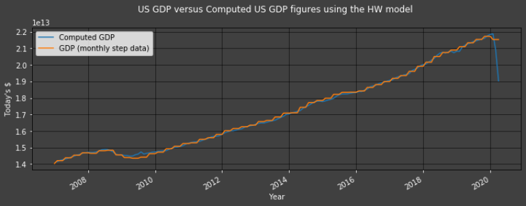
Conclusion
It is possible to estimate monthly US GDP figures using the HW model to a good degree of accuracy. The final forecast even anticipated the fall in GDP caused by COVID-19 (in 2020) before official figures were released. Such estimates can not only be done via an Expenditure Approach but also an Income Approach; a mixture of the two would be an interesting study.
Note that it is possible to use this method to compute future monthly GDP forecasts.
References:
Mitchell, Smith, Weale, Wright, and Salazar (2005): James Mitchell, Richard J. Smith, Martin R. Weale, Stephen Wright, Eduardo L. Salazar, An Indicator of Monthly GDP and an Early Estimate of Quarterly GDP Growth, The Economic Journal, Volume 115, Issue 501, February 2005, Pages F108–F129, https://doi.org/10.1111/j.0013-0133.2005.00974.x
Video Tutorials