Author:

The Datastream Commodities Overview illustrates recent price movements for key commodities in the Metals, Energy, Chemicals, Agriculture, and Indices. It uses DataStream Web Services to retrieve the one-year historical price for commodities and then plot line charts with trend lines that demonstrate directions and movements of prices. It also shows summary data such as, percentage change, one year low, and one year high in the table. It is similar to the Datastream Commodities Overview in the Refinitiv Eikon Excel Template Library.
Datastream
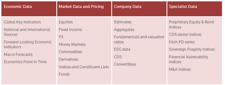
Datastream is the world’s leading time-series database, enabling strategists, economists, and research communities’ access to the most comprehensive financial information available. With histories back to the 1950s, you can explore relationships between data series; perform correlation analysis, test investment and trading ideas, and research countries, regions, and industries.
The Datastream database has over 35 million individual instruments or indicators across major asset classes. You can directly invoke the web service methods from your applications by using the metadata information we publish.
The Datastream Web Service allows direct access to historical financial time series content listed below.
For more information, please refer to Datastream Web Service.
DatastreamDSWS
This example uses the DatastreamDSWS library to connect and retrieve data from Datastream. To use this Python library, please refer to the Getting Started with Python document.
Loading Libraries
The required packages for this example are:
- DataStreamDSWS: Python API package for Refinitiv Datastream Webservice
- matplotlib: A comprehensive library for creating static, animated, and interactive visualizations in Python
- pandas: Powerful data structures for data analysis, time series, and statistics
- dateutil: Powerful extensions to the standard datetime module
- ipywidgets: IPython HTML widgets for Jupyter
- numpy: The fundamental package for array computing with Python
import numpy as np
import matplotlib.pyplot as plt
import dateutil
import matplotlib.dates as mdates
import DatastreamDSWS as DSWS
import pandas as pd
import ipywidgets as widgets
from ipywidgets import Button, HBox, VBox, Dropdown, Label, Layout
Setting Credentials
The DataStream username and password are required to run the example.
ds = DSWS.Datastream(username = '<username>', password = '<password>')
Specifying Data Types and Expressions
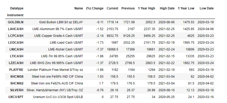
The following fields are displayed in the summary table.
| Data Types or Expressions | Descriptions |
|---|---|
| NAME | The name of the equity/company or equity list, as stored on Datastream’s databases |
| PCH#(X,-1D) | The percent change percent from yesterday to today |
| X | Today's price| |
| VAL#(X,-1D) | Yesterday's price| |
| MAX#(X,-1Y) | The highest price within one year |
| MAXD#(X,-1Y) | The date of the highest price| |
| MIN#(X,-1Y) | The lowest price within one year |
| MIND#(X,-1Y) | |The date of the lowest price |
The variable is specified as a class. The keys contain the data types or expressions and the values contain descriptions.
You can access the Datastream Navigator to search for data types or instruments. For other expressions, refer to the Datastream help page.
summary_fields = {
'NAME':'Name',
'PCH#(X,-1D)':'(%) Change',
'X':'Current',
'VAL#(X,-1D)':'Previous',
'MAX#(X,-1Y)':'1 Year High',
'MAXD#(X,-1Y)':'High Date',
'MIN#(X,-1Y)':'1 Year Low',
'MIND#(X,-1Y)':'Low Date'
}
Specifying Instruments
Next, I specify instruments of key commodities in the Metals, Energy, Chemicals, Agriculture, and Indices.
Metals
| Instruments | Descriptions |
|---|---|
| GOLDBLN | Gold Bullion LBM $/t oz DELAY |
| SILVERH | Silver, Handy&Harman (NY) U$/Troy OZ |
| PLATFRE | London Platinum Free Market $/Troy oz |
| LAHCASH | LME-Aluminium 99.7% Cash U$/MT |
| LCPCASH | LME-Copper Grade A Cash U$/MT |
| LEDCASH | LME-Lead Cash U$/MT |
| LNICASH | LME-Nickel Cash U$/MT |
| LTICASH | LME-Tin 99.85% Cash U$/MT |
| LZZCASH | LME-SHG Zinc 99.995% Cash U$/MT |
| SHCNI62 | Steel Iron ore Fe62% AUS CIF China |
| SHCNI58 | Steel Iron ore Fe58% IND CIF China |
| UXCUSPT | Uranium UxC-Ux U3O8 Spot U$/LB |
Energy
| Instruments | Descriptions |
| OILBREN | Crude Oil BFO M1 Europe FOB $/BBl |
| OILWTXI | Crude Oil WTI NYMEX Close M U$/BBL |
| GASUREG | Gasoline,Unld. Reg. Oxy. NY Cts/Gal |
| DIESELA | Diesel, .05% Sulphur LA C/GAL |
| JETCIFC | Jet Kerosene-Cargos CIF NWE U$/MT |
| FUELOIL | Fuel Oil No.2 (New York) C/Gallon |
| OILGASO | Gas Oil-EEC CIF Cargos NWE U$/MT |
| OILNAPH | Naphtha Europe CIF U$/MT |
| NATBGAS | ICE Natural Gas 1 Mth.Fwd. P/Therm |
| LMCYSPT | Coal ICE API2 CIF ARA Nr Mth $/MT |
| EEXPEAK | EEX - Phelix Peak Hr.09-20 E/Mwh |
| ES15PSN | SNL US Electricity Peak load SP-15 |
Chemicals
| Instruments | Descriptions |
|---|---|
| ETYEUSP | Ethylene,Eur Spot FD NWE Pipe E/MT |
| PPPEUSF | Propylene (P),Spot FD NWE E/MT |
| STYEUSP | Styrene,Spot FOB Rdam T2 U$/MT |
| PVCUSDG | PVC,USG Domestic GP UC/LB |
| PLYEUSP | Polye HDPE Bl/Mldg, NWE Spot FD E/KG |
| PLLEUSO | Polye LLDPE,Europe Spot OCT. E/KG |
| PLPEUSN | PP Copolymer,Spot FD NWE E/KG |
| PLSEUDM | Polystyrene-GP, Dom FD UK £/MT |
| PTANWEC | PTA,Contract FD NWE E/MT |
| SODNWED | Caustic Soda, Liquid FOB NWE U$/DMT |
| UREAGRN | Urea Granular CFR New Orleans $/MT |
| DAPNOCB | DAP, New Orleans CFR Barge U$/MT |
Agriculture
| Instruments | Descriptions |
|---|---|
| GSCITOT | S&P GSCI Commodity Total Return |
| DJUBSTR | Bloomberg- Commodity TR |
| RICIXTR | Rogers International Commodity Ind TR |
| CYDMNTR | CYD Market Neutral+ Total Return |
| RJEFCRT | RF/CC CRB TR |
| MLCXTOT | MLCX Total Return |
| DBKLCIX | DBLCI Optimum Yield Diversifi ER Idx |
| BALTICF | Baltic Exchange Dry Index (BDI) |
| LMEINDX | LME-LMEX Index |
| DRAMDXI | DRAMeXchange-DXI Index |
Commodities Indices
| Instruments | Descriptions |
|---|---|
| GSCITOT | S&P GSCI Commodity Total Return |
| DJUBSTR | Bloomberg- Commodity TR |
| RICIXTR | Rogers International Commodity Ind TR |
| CYDMNTR | CYD Market Neutral+ Total Return |
| RJEFCRT | RF/CC CRB TR |
| MLCXTOT | MLCX Total Return |
| DBKLCIX | DBLCI Optimum Yield Diversifi ER Idx |
| BALTICF | Baltic Exchange Dry Index (BDI) |
| LMEINDX | LME-LMEX Index |
| DRAMDXI | DRAMeXchange-DXI Index |
All instruments and summary fields are set into the commodities variable with categories as key names.
{'Metals': {'Items': ['GOLDBLN', 'SILVERH', ...], 'Fields': {'NAME': 'Name', 'PCH#(X,-1D)': '(%) Change', ...}}, 'Energy': {'Items': ['OILBREN', 'OILWTXI', ...], 'Fields': {'NAME': 'Name', 'PCH#(X,-1D)': '(%) Change', ...}}, 'Chemicals': {'Items': ['ETYEUSP', 'PPPEUSF', ...], 'Fields': {'NAME': 'Name', 'PCH#(X,-1D)': '(%) Change', ...}}, 'Argiculture': {'Items': ['WHEATSF', 'CORNUS2', ...], 'Fields': {'NAME': 'Name', 'PCH#(X,-1D)': '(%) Change', ...}}, 'Indices': {'Items': ['GSCITOT', 'DJUBSTR', ...], 'Fields': {'NAME': 'Name', 'PCH#(X,-1D)': '(%) Change', ...}}} |
commodities = {}
# Metals
commodities['Metals'] = {}
commodities['Metals']['Items']=[
'GOLDBLN','SILVERH','PLATFRE','LAHCASH',
'LCPCASH','LEDCASH','LNICASH','LTICASH',
'LZZCASH','SHCNI62','SHCNI58','UXCUSPT']
commodities['Metals']['Fields']=summary_fields
# Energy
commodities['Energy'] = {}
commodities['Energy']['Items']=[
'OILBREN','OILWTXI', 'GASUREG','DIESELA',
'JETCIFC','FUELOIL','OILGASO','OILNAPH',
'NATBGAS','LMCYSPT','EEXPEAK','ES15PSN']
commodities['Energy']['Fields']=summary_fields
# Chemicals
commodities['Chemicals'] = {}
commodities['Chemicals']['Items']=[
'ETYEUSP','PPPEUSF','STYEUSP','PVCUSDG',
'PLYEUSP','PLLEUSO','PLPEUSN','PLSEUDM',
'PTANWEC','SODNWED','UREAGRN','DAPNOCB']
commodities['Chemicals']['Fields']=summary_fields
# Argiculture
commodities['Argiculture'] = {}
commodities['Argiculture']['Items']=[
'WHEATSF','CORNUS2','RIT1STA','WOLAWCE',
'WSUGDLY','COCINUS','COTTONM','SOYBEAN',
'PAOLMAL','CLHINDX','USTEERS','MILKGDA']
commodities['Argiculture']['Fields']=summary_fields
#Commodities Indices
commodities['Indices'] = {}
commodities['Indices']['Items']=[
'GSCITOT','DJUBSTR','RICIXTR','CYDMNTR',
'RJEFCRT','MLCXTOT','DBKLCIX','BALTICF',
'LMEINDX','DRAMDXI']
commodities['Indices']['Fields']=summary_fields
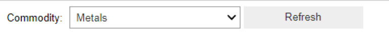
Defining a Widget to Display Commodities Overview
In this section, we will create a widget that displays Commodities Overview of a selected commodities' category (Metals, Energy, Chemicals, Agriculture, and Indices). After selecting the category, the widget uses the get_data method in the DataStreamDSWS library to retrieve daily historical prices for one year of the instruments in the selected category.
| ds.get_data (tickers="GOLDBL,SILVERH,PLATFRE,LAHCASH, LCPCASH,EDCASH,LNICASH,LTICASH, LZZCASH,SHCNI62,SHCNI58,UXCUSPT", start='-1Y') |
Then, it uses the matplotlib library to plot historical charts with trend lines of the returned prices.
Next, it calls the get_data method to retrieve the data for the summary fields and then displays the data in tabular format.
ds.get_data(tickers="GOLDBL,SILVERH,PLATFRE,LAHCASH, LCPCASH,EDCASH,LNICASH,LTICASH, LZZCASH,SHCNI62,SHCNI58,UXCUSPT", fields=['NAME','PCH#(X,-1D)','X', 'VAL#(X,-1D)','MAX#(X,-1Y)','MAXD#(X,-1Y)', 'MIN#(X,-1Y)','MIND#(X,-1Y)'], kind=0) |
class CommodityOverviewWidget:
status_label = Label("")
cache = {}
title_label = Label(value='')
button = Button(description='Refresh')
output = widgets.Output()
commodity_dropdown = None
def __init__(self, _context):
dropdown_options = list(_context.keys())
self.commodity_dropdown = Dropdown(options=dropdown_options, value=dropdown_options[0],description='Commodity:')
display(HBox([self.commodity_dropdown, self.button]),
self.output)
self.button.on_click(self.on_button_clicked)
self.commodity_dropdown.observe(self.on_change)
self._context = _context
def display_data(self, name, static_data, df):
with self.output:
display(VBox([Label(r'\(\bf{'+ name +r'}\)')]
,layout=Layout(width='100%', display='flex' ,
align_items='center')))
dates = [dateutil.parser.parse(x) for x in df.index]
X = mdates.date2num(dates)
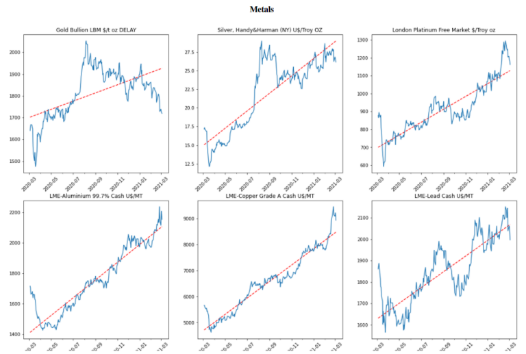
fig, axs = plt.subplots(nrows=4, ncols=3,figsize=(20, 20))
plt.close(fig)
fig.subplots_adjust(top = 2)
fig.subplots_adjust(bottom = 1)
for index in range(df.shape[1]):
z = np.polyfit(X, np.array(df.iloc[: , index].values), 1)
p = np.poly1d(z)
ax = axs[int(index/3), int(index%3)]
ax.plot(X,p(X),"r--")
ax.plot(X, df.iloc[: , index].values)
loc= mdates.AutoDateLocator()
years = mdates.YearLocator() # every year
months = mdates.MonthLocator() # every month
years_fmt = mdates.DateFormatter('%Y-%m')
ax.set_title(static_data.loc[df.iloc[: , index].name[0]]['Name'])
ax.xaxis.set_major_formatter(years_fmt)
ax.xaxis.set_minor_locator(months)
ax.xaxis.set_major_locator(loc)
for tick in ax.get_xticklabels():
tick.set_rotation(45)
self.output.clear_output()
display(VBox([Label(r'\(\bf{'+ name +r'}\)')]
,layout=Layout(width='100%', display='flex' ,
align_items='center')))
display(fig)
display(static_data)
def on_change(self, change):
if change['type'] == 'change' and change['name'] == 'value':
if change['new'] not in self.cache or self.cache[change['new']] == {}:
self.refresh_data(change['new'])
else:
self.display_data(change['new'], self.cache[change['new']]['static'], self.cache[change['new']]['df'])
def refresh_data(self, name):
commodity = self._context[name]
itemList = commodity['Items']
fieldList = commodity['Fields']
with self.output:
self.output.clear_output()
self.status_label.value="Running..."
display(self.status_label)
df = ds.get_data (tickers=",".join(itemList), start='-1Y') #kind=1
df.dropna(inplace=True)
static_data = ds.get_data(tickers=",".join(itemList),fields=list(fieldList.keys()), kind=0)
static_data = static_data.pivot(index='Instrument', columns='Datatype')["Value"]
static_data = static_data[list(fieldList.keys())].rename(columns=fieldList)
self.cache[name]={}
self.cache[name]['static']=static_data
self.cache[name]['df']=df
self.display_data(name, static_data, df)
def on_button_clicked(self,c):
self.refresh_data(self.commodity_dropdown.value)
The output looks like the following.
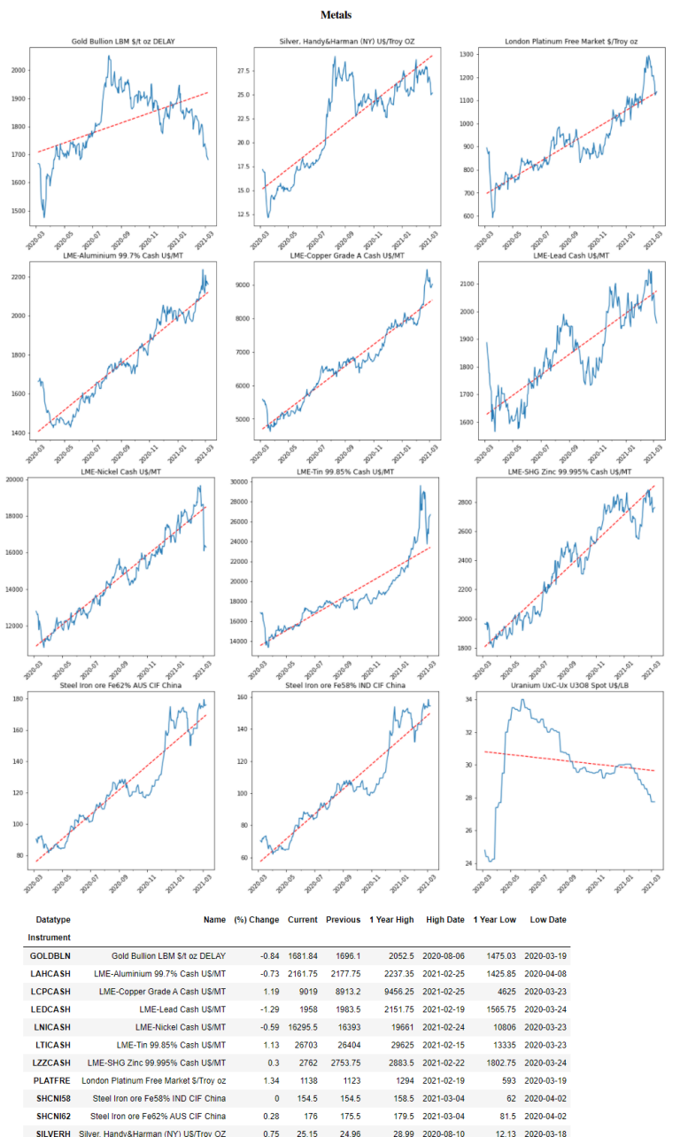
CommodityOverviewWidget(commodities)
References
- Developers.refinitiv.com. 2021. Datastream Web Service | Refinitiv Developers. [online] Available at: https://developers.refinitiv.com/en/api-catalog/eikon/datastream-web-service [Accessed 5 March 2021].
- Kumar, A., 2020. Python: How to Add a Trend Line to a Line Chart/Graph - DZone Big Data. [online] dzone.com. Available at: https://dzone.com/articles/python-how-to-add-trend-line-to-line-chartgraph [Accessed 5 March 2021].
- Product.datastream.com. 2020. Datastream Login. [online] Available at: http://product.datastream.com/browse/ [Accessed 12 June 2020].
Source Code