
Article
Multi-factor approach to understanding a portfolio's country risk exposure


How do you assess your portfolio’s risk exposure when the entities you invest in are international, complex and face a multitude of regulatory challenges? How do you assess the risk exposure to a company that is headquartered in a relatively “safe” country, but has key subsidiaries spread across more volatile, less-known locations?
By utilizing country risk models, we can provide a new and bigger picture of your portfolio’s country risk exposure. The following article will draw on these risk factors and weigh your portfolio’s investment strategy based on key factors such as the revenue distribution and the location of the company’s headquarters to highlight your investment exposure.
Getting Started
For this analysis, we plan to utilize data and the associated models available available within LSEG's comprehensive data set. To get started we will need to import the Refinitiv Data (RD) Library responsible for risk predictions. In addition, we'll use some popular charting packages to highlight the risk exposure based on our portfolio of holdings.
import refinitiv.data as rd
import pandas as pd
import numpy as np
import matplotlib.pyplot as plt
import plotly.graph_objects as go
plt.style.use('dark_background')
# Open a session into the desktop. The session represents the interface to extract our risk data.
rd.open_session()
Process Workflow
The following workflow outlines concrete steps involved in evaluating the risk exposure for a given portfolio of holdings. The steps have been intentionally broken out into well-defined segments for the purposes of reusability as well as a basis for understanding the processing details.
- Portfolio Definition
To simplify the algorithm, the following notebook will assume an existing portfolio has been defined within the Eikon or Refinitiv Workspace desktop application. The portfolio definition provides the user multiple options to pull in specific details related to the holdings within the portfolio. Users can create their own portfolios, define the list of companies and the holdings for each, and can generate a risk factor breakdown based on country. - Clean the Portfolio
When constructing a portfolio, there may be instances where some of the positions may not define a risk factor, for example, cash. To analyze our exposure, we need to remove these holdings to properly weigh and calculate risk within each country. - Data Preparation
With a clean portfolio, we'll need to prepare the data set by calculating the risk, based on a weighted factor. Because we may have removed holdings from our data set, this will require an adjustment to the weight of each position. Coupled with the StarMines' risk factor calculation, we can prepare the a weighted risk across the portfolio. - Visualization and Analysis
Finally, we can put it all together by bucketing our results into a suitable generation of charts showing a breakdown of risk across each country and where the greatest exposure exists.
1. Portfolio Definition
To analyze the exposure of your holdings, we can utilize the risk factors defined within the StarMine Countries of Risk model. For our analysis, we assume the user has utilized the power of the PAL (Portfolios & Lists) manager app defined within the Eikon or Refinitiv Workspace desktop application. Users simply create the list of instruments and what they are holding. The PAL app assigns a weighted factor based on the market value of each holding. Coupled with these calculated values, we can utilize the capabilities of the StarMine database to pull down the risk factors and country details. These measures will represent the basis of our analysis.
StarMine Countries of Risk Model
Available to the user are a number relevant properties required to analyze risk based on where the company does business. For our analysis, we are pulling down the following:
- Countries of Risk Fraction
The fractional exposures allocated to the top 10 countries of risk. While many companies do business in more than 10 countries, it is entirely possible the list of countries may be limited to 1 or only a few participating countries. - The name of the country
The list of the top 10 countries for each portfolio holding. These countries are used to highlight the distribution of holdings to evaluate our exposure.
The StarMine Countries of Risk Model uses four sources of data, which are, in order of importances:- Revenue distribution by geography
- The location of a company's headquarters
- The country where its primary equity security listing trades
- Financial reporting currency
The model provides estimates on the countries to which a company is exposed, and estimates a fractional contribution to each. The higher the value, the higher exposure to the country.
# Retrieve our portfolio and specify the risk factors for each
fields = ['TR.PortfolioConstituentName','TR.PortfolioWeight', 'TR.CoRFractionByCountry',
'TR.CoRFraction','TR.CoRFraction.countryname']
# Choose a portfolio (Users simply change the value below to reflect their defined portfilio)
data = rd.get_data('Portfolio(SAMPLE_GL_DEV)', fields)
By utilizing the 'Portolio()' syntax, the library will take care of extracting and pulling in multiple attributes specific to the referenced portfolio, in particular, the risk factors.
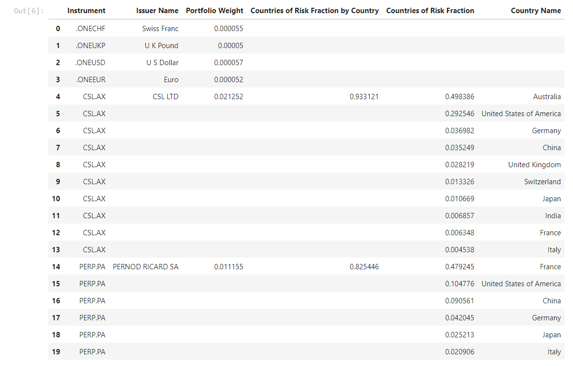
# Provide a quick snapshot to show what we captured
data.head(20)
2. Clean the Portfolio
In the above portfolio, we can see a partial list of instruments, a breakdown of the risk factors for the top 10 countries and the weight of each instrument within the portfolio. However, it may be possible the portfolio contains instruments that are not susceptible to exposure, for example cash, and thus will not carry any risk. As such, we need to clean out this data. As a result, the weights may be skewed and thus will need to be normalized after we clean the data.
# Remove all rows/entries where we are missing relevant data.
# The missing data within our risk column needs to be removed.
data.dropna(inplace=True, subset=['Countries of Risk Fraction'])
Depending on the selected portfolio, there may be many positions removed or none at all.
3. Data Preparation
- Adjusted Weight
Because we potentially removed positions within our portfolio, we'll need to adjust each positions weight relative to the new portfolio. - Weighted Risk
Based on the adjusted weight of each holdings and StarMines' country of risk fraction, calculate a weighted risk value for each country per Instrument. - Group Country factors
The goal of our analysis is to highlight the total risk exposure within a country, based on our holdings. We do this by grouping our country weighted risk factors across all holdings.
Adjusted Weight
# Calculate the adjusted weight factor...
adjusted_weight_factor = data['Portfolio Weight'].sum()
# Then use this value to created a new 'Adjusted Weight' value for our collection
data['Adjusted Weight'] = data['Portfolio Weight'].transform(lambda x: x / adjusted_weight_factor)
# Show the new 'adjusted weight' calculation...
data.head(20)
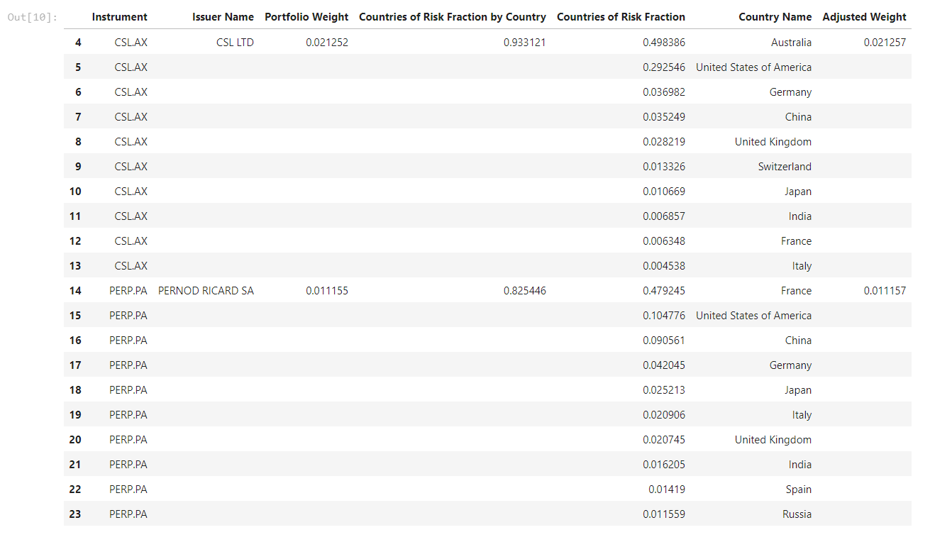
With our portfolio clean, the above table shows the positions that have been removed and a newly adjusted weight for our updated portfolio.
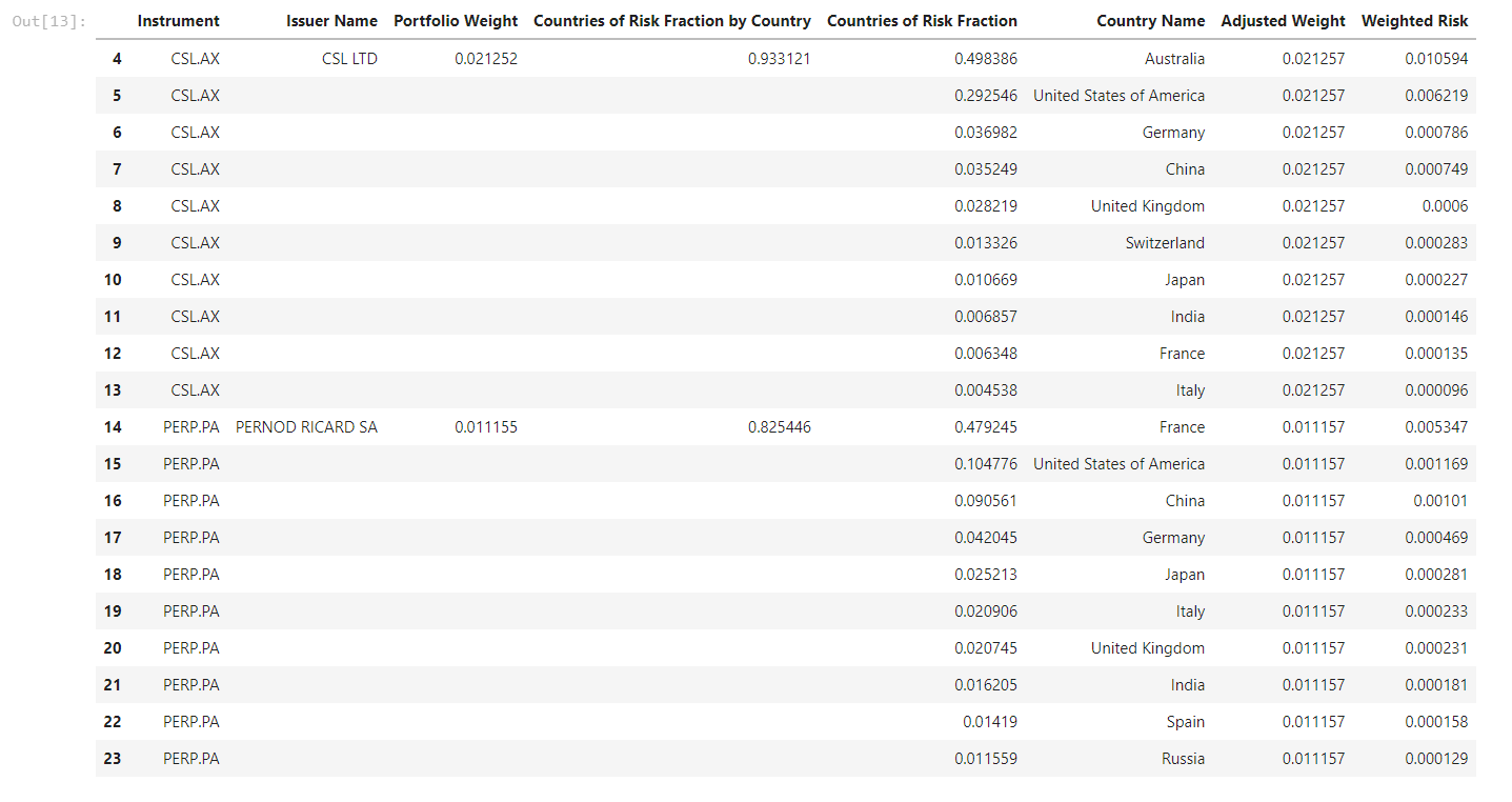
Weighted Risk
The Weighted Risk represents the risk based on our holdings for each position and the risk factor defined. This value will act as the basis to determine the exposure for each country. The following represents the details around this calculated value:
# Prior to calculating the 'weighted risk', we need to backfill the Adjusted weights...
adj_weight = 'Adjusted Weight'
data.loc[:,adj_weight] = data.loc[:, adj_weight].ffill(axis=0)
# Calculate our weighted risk
data['Weighted Risk'] = data[adj_weight] * data['Countries of Risk Fraction']
data.head(20)
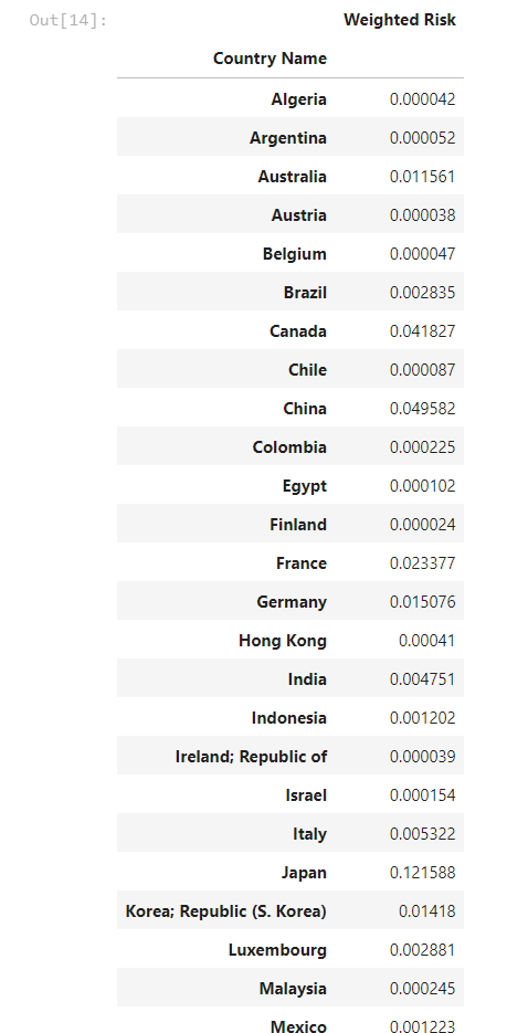
# Bucket the total weighted risk across our portfolio, grouped by country
group = data.groupby('Country Name')['Weighted Risk'].sum().to_frame()
group
# First, normalize the factors to represent %100 coverage...
adjusted_risk_factor = group['Weighted Risk'].sum()
group['Adjusted Weighted Risk'] = group['Weighted Risk'].transform(lambda x: x / adjusted_risk_factor)
# Sort the table to highlight the countries with the greatest exposure
result = group.sort_values(by='Adjusted Weighted Risk', ascending=False)
# Prepare
result.reset_index(level=0, inplace=True)
# Output a tabular display of our exposure sorted based on the highest risk
result
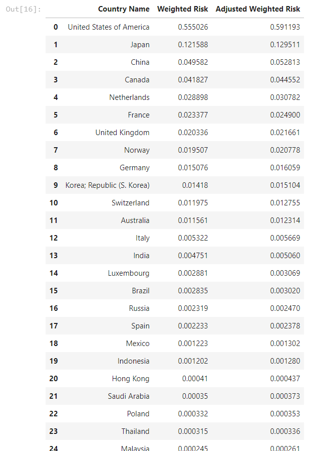
Presentation
For simplicity, we've defined a couple of presentation displays, bar and pie chart, representing a way to easily highlight countries with the greatest exposure:
# Bar graph function showing exposure
def bar(data):
plt.rcParams['figure.figsize'] = (13,7)
fig, ax = plt.subplots()
ax.tick_params(labelrotation=90)
ax.bar(
x = np.arange(data.shape[0]),
height = data['Adjusted Weighted Risk'],
tick_label=data['Country Name'],
alpha=0.5
)
# Remove the borders from the graph - leave the bottom
ax.spines['top'].set_visible(False)
ax.spines['right'].set_visible(False)
ax.spines['left'].set_visible(False)
ax.tick_params(bottom=False, left=False)
# Add a faint grid
ax.yaxis.grid(True, alpha=0.1)
ax.xaxis.grid(True, alpha=0.1)
# Add labels and a title. Note the use of `labelpad` and `pad` to add some
# extra space between the text and the tick labels.
ax.set_ylabel('Risk Factor', labelpad=15, fontsize=16, color='cyan')
ax.set_title("Portfolio Country Risk Exposure", pad=15, fontsize=16, color='cyan')
fig.tight_layout()
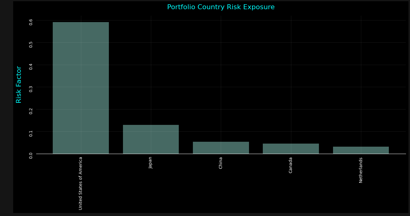
# Show to top 5...
bar(result.head())
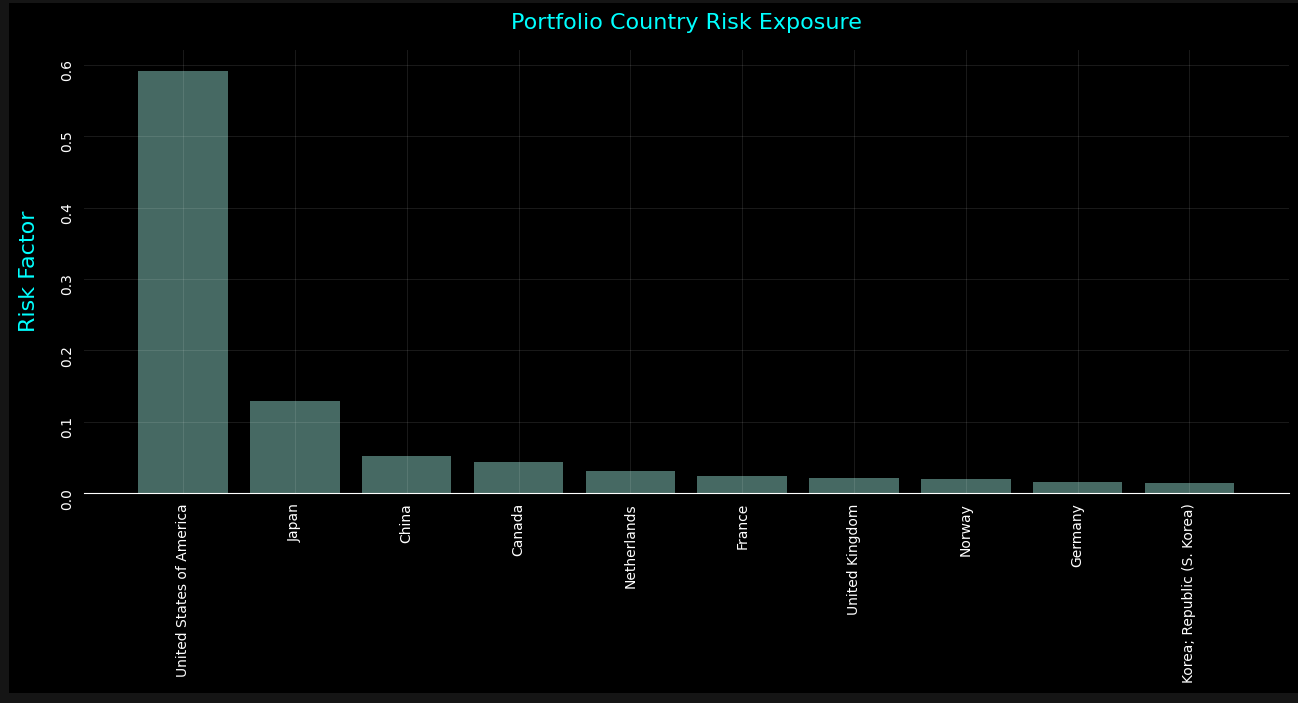
# Top 10...
bar(result.head(10))
# Pie Chart function showing exposure
def pie(data):
labels = data['Country Name'].tolist()
values = data['Adjusted Weighted Risk'].tolist()
# Use `hole` to create a donut-like pie chart
fig = go.Figure(data=[go.Pie(labels=labels, values=values, hole=.3)])
fig.update_layout(
font={
'size': 9,
'color': 'cyan'
},
margin={
't': 50,
'b': 0,
'r': 0,
'l': 0,
'pad': 0,
},
title={
'text': f'Portfolio Country Risk Exposure',
'y': 0.95,
'x': 0.425
},
titlefont={
'size': 20,
'color': 'cyan'
},
paper_bgcolor='rgba(0,0,0,0)'
)
fig.show()
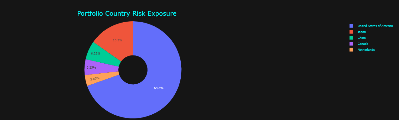
# Show to top 5...
pie(result.head())
# Top 10...
pie(result.head(10))
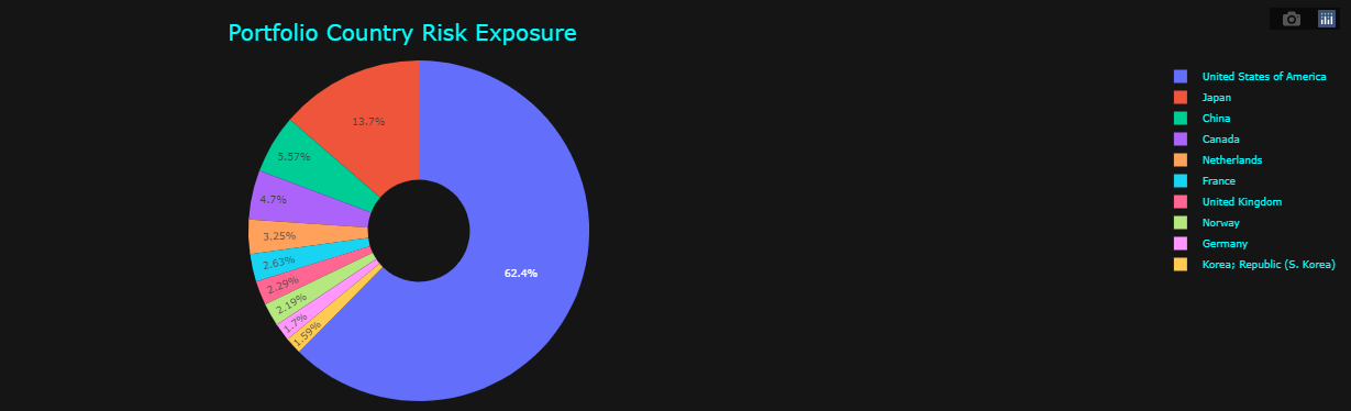
The above presentation clearly highlights and breaks down the countries where the greatest exposure may be. The models are designed to provide a general guidance. As such, the analysis is meant to generalize exposure based on the weighting of each position within the portfolio and how these positions are affected by the countries where business occurs.
Conclusion
The StarMine Countries Of Risk data removes the incertitude and complexity of getting a bigger picture of the portfolio risk exposure using unbiased and verifiable data. It simplifies the intricacy of global entities while providing a full representation of risk exposure . Looking at your portfolio asset allocation by country of exchange or headquarter may omit the underlying exposure risks that could affect your portfolio’s performance and constraints.
Source Code
Documentation
Related APIs