Author:

In this article, we build a data-frame to output an instrument's Daily (i) Close Prices, (ii) ln (logarithme naturel / natural logarithm) Return, (iii) Close Price's 10, 30 and 60 Day Moving Averages, (iv) Close Price's ln Return 10, 30 and 60 Day Moving Average, (v) Annualised Standard Deviation (i.e.: volatility) of the 10, 30 and 60 Day Rolling Window (Natural Log) Returns (based on CLOSE prices), and (vi) Relative Strength Index (RSI).
When it comes to the RSI data, a great article to read about its implementation can be found here (thank you Umer and Jason!). You may want to read into the installation of the TA-Lib library used to compute RSI data here. You may also want to read into how the way TA-lib calculates RSI; as per its GitHub documentation, it uses a Wilder Smoothing method to compute Moving Averages. Others may use different such methods (e.g.: Exponential Moving Average or Simple Moving Average). More information on Refinitiv Workspace's Chart App RSI can be found here and here. Previous RSI Python functions do not provide great amounts of customisation; in this article, we will create a Python function that does just that.
Webinar Video
This Webinar was broadcasted live on Twitch where I code live every Tuesday at 4pm GMT.
Using this Site
You may scale up or down the math figures at your convenience as per the below.

Relative Strength Index
The Relative Strength Index (RSI) is a value between 0 and 100 calculated for any one asset based on its historical price; it indicates an asset as oversold if bellow a certain threshold - idest (i.e.): it's underpriced - and overbought if above a certain threshold - i.e.: it's overpriced. RSI at time $t$ is calculated $RSI_{w, m, t}$ where $w$ is the window asked for (e.g.: 14) and where $m$ is either (i) $SMA$ (Simple Moving Average) or $Cutler$, (ii) $EMA$ (Exponential Moving Average), or (iii) $Wilder$ or $MEMA$ (Modified Exponential Moving Average):
(i) with $SMA$ (Simple Moving Average) or $Cutler$ such that $m_1=\{SMA, Cutler\}$: $$ RSI_{w, m_1, t} = \begin{Bmatrix} 100 & \text{if } \sum_{i=1}^w{|min(P_{t-i+1} - P_{t-i} \text{ }, \text{ } 0)|} = 0 \\ 100 - \frac{100}{ 1 +\frac{ \sum_{i=1}^w{max(P_{t-i+1} - P_{t-i} \text{ }, \text{ } 0)}} {\sum_{i=1}^w{|min(P_{t-i+1} - P_{t-i} \text{ }, \text{ } 0)|}} } & \text{otherwise} \end{Bmatrix} $$
(ii) & (iii) with $EMA$, or $Wilder$ / $MEMA$ such that $m_2=\{EMA, Wilder, MEMA\}$:
$$ RSI_{w, m_2, 1} = RSI_{w, m_1, 1} $$and
$$ RSI_{w, m_2, \tau} = 100 - \frac{100}{ \left[ 1 + \frac{ a_m * \left( max(P_{\tau} - P_{\tau-i} \text{ }, \text{ } 0) \right) + (1 - a_m) * \left( \sum_{i=1}^w{max(P_{\tau-i+1} - P_{\tau-i} \text{ }, \text{ } 0)} \right)}{ a_m * \left( |min(P_{\tau} - P_{\tau-1} \text{ }, \text{ } 0)| \right) + (1 - a_m) * \left( \sum_{i=1}^w{|min(P_{\tau-i+1} - P_{\tau-i} \text{ }, \text{ } 0)|} \right)} \right]} $$where $\tau > 1$, and
$$ a_m = \begin{Bmatrix} a_{MEMA} = a_{Wilder} = & \frac{1}{w} & \text{if } m \text{ is } MEMA \text{ or } Wilder \\ a_{EMA} = & \frac{2}{w + 1} & \text{if } m = EMA \end{Bmatrix} $$And it is computed as such:
start_date, end_date, bdpy = '2020-01-01', '2021-08-01', 360 # ' bdpy ' stands for 'business days per year'
maws = [10, 30, 60] # ' maws ' stands for 'moving average windows'
rsiw = 14
rsi_method = "Wilder" # "SMA", "EMA", "Wilder"
ric_list = ['KO.N', 'VOD.L']
from datetime import datetime
from dateutil.relativedelta import relativedelta # '2.8.1'
import numpy # '1.18.2'
import statistics
import pandas # '1.2.4'
pandas.set_option('display.max_columns', None) # This allows us to see all the collumns of our dataframe
import eikon as ek
# The key is placed in a text file so that it may be used in this code without showing it itself:
eikon_key = open("eikon.txt", "r")
ek.set_app_key(str(eikon_key.read()))
# It is best to close the files we opened in order to make sure that we don't stop any other services/programs from accessing them if they need to:
eikon_key.close()
df1, err = ek.get_data(
instruments=ric_list,
fields=['TR.PriceClose.date', 'TR.PriceOpen', 'TR.PriceClose', 'TR.VOlume'], # could also have TR.RSISimple30D & TR.RSISimple14D
parameters={'SDate': start_date, 'EDate': end_date})
# Step 1: Create a list of days ranging throughout our period.
# The reason we look at every day is because some securities might trade on Sunday (e.g.: in middle-east)
delta = datetime.strptime(end_date, '%Y-%m-%d') - datetime.strptime(start_date, '%Y-%m-%d')
days = [datetime.strptime(start_date, '%Y-%m-%d') + relativedelta(days=i)
for i in range(delta.days + 1)]
# Step 2: Create a pandas data-frame to populate with a loop
df2 = pandas.DataFrame(index=days)
# Step 3: Create a loop to populate our 'df' dataframe
# for m, i in enumerate(ric_list):
for i in ric_list:
# get Close Prices: (You may use any way to collect such data, here we are recycling previous data)
_df = pandas.DataFrame(
data=[float(j) for j in df1[df1["Instrument"] == i]["Price Close"]],
columns=[f"{i} Close"],
index=[datetime.strptime(df1[df1["Instrument"] == i]["Date"][j],
'%Y-%m-%dT%H:%M:%SZ')
for j in list(df1[df1["Instrument"] == i]["Date"].index)])
# get ln (logarithme naturel) return from Close Prices:
_df[f"{i}'s ln Return"] = numpy.log(
_df[f"{i} Close"] / _df[i + " Close"].shift(1))
# get 1st difference in Close Prices:
dCP = list((_df[f"{i} Close"] - _df[f"{i} Close"].shift(1)))
# dCP.insert(0, numpy.nan)
# list.reverse(dCP)
_df[f"{i}'s 1d Close"] = dCP
for j in maws:
# get Close Price's 10, 30 and 60 Day Moving Averages
_df[f"{i}'s Close {str(j)}D MA"] = _df[f"{i} Close"].dropna().rolling(j).mean()
# get Close Price's ln Return 10, 30 and 60 Day Moving Average
_df[f"{i}'s ln Return' {str(j)}D MA"] = _df[f"{i}'s ln Return"].dropna().rolling(j).mean()
# # You may also want to look into TA-lib's Simple Moving Average function:
# _df[i + "'s ln Return' " + str(j) + " Day Moving Average"] = ta.SMA(_df[i + " Close"], j)
# get Annualised Standard Deviation (i.e.: volatility) of the 10, 30 and 60 Day Rolling Window (Natural Log) Returns (based on CLOSE prices)
_df[f"{i}'s Ann. S.D. of {str(j)}D Roll. of ln Returns"] = _df[f"{i}'s ln Return"].dropna().rolling(j).std()*(bdpy**0.5)
# RSI: Simple Moving Average
if rsi_method == "SMA" or rsi_method == "Cutler":
RSIw = []
for k in range(len(dCP) - rsiw):
up_moves, down_moves = [], []
for j in range(k, k + rsiw):
up_moves.append(max(dCP[j + 1], 0)) # ' + 1 ' because we're looking at 1st difference data, the 1st element of which is always nan.
down_moves.append(abs(min(dCP[j + 1], 0))) # ' + 1 ' because we're looking at 1st difference data, the 1st element of which is always nan.
AvgU = statistics.mean(up_moves)
AvgD = statistics.mean(down_moves)
if AvgD == 0:
RSIw.append(100)
else:
RSw = AvgU/AvgD
RSIw.append(100-(100/(1+RSw)))
# RSI: Exponential Moving Average
if rsi_method == "EMA" or rsi_method == "MEMA" or rsi_method == "Wilder":
if rsi_method == "MEMA" or rsi_method == "Wilder":
a = 1 / rsiw
elif rsi_method == "EMA":
a = 2 / (rsiw + 1)
RSIw, up_moves, down_moves = [], [], []
for k in dCP[1:]: # ' [1:] ' because we're looking at 1st difference data, the 1st element of which is always nan.
up_moves.append(max(k, 0))
down_moves.append(abs(min(k, 0)))
AvgU = [statistics.mean(up_moves[0:rsiw])]
AvgD = [statistics.mean(down_moves[0:rsiw])]
if AvgD[0] == 0:
RSIw.append(100)
else:
RSw = AvgU[0] / AvgD[0]
RSIw.append(100 - (100 / (1 + RSw)))
for k in range(rsiw, len(up_moves)):
AvgU.append(a * up_moves[k] + (1 - a) * AvgU[k - rsiw])
AvgD.append(a * down_moves[k] + (1 - a) * AvgD[k - rsiw])
RSw = AvgU[k - rsiw] / AvgD[k - rsiw]
RSIw.append(100 - (100 / (1 + RSw)))
RSIw.append(numpy.nan) # This is needed to inser the nan from the 1st difference that was already nan
for k in range(len(_df.index) - len(RSIw)):
RSIw.insert(0, numpy.nan)
_df[f"{i}'s RSI{rsiw}"] = RSIw
# Finally: merge all.
df2 = pandas.merge(
df2, _df, how="outer", left_index=True, right_index=True)
display response
import plotly
import plotly.express
from plotly.graph_objs import *
from plotly.offline import download_plotlyjs, init_notebook_mode, plot, iplot
init_notebook_mode(connected=True)
import cufflinks
cufflinks.go_offline()
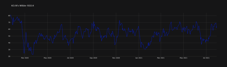
df2["KO.N's RSI14"].dropna().iplot(title="KO.N's Wilder RSI14",
colors="#001EFF", theme="solar")
Define a Python Function
def Refinitiv_RSI(start_date='2020-01-01', end_date='2021-08-01', bdpy=360, # ' bdpy ' stands for 'business days per year'
maws=[10, 30, 60], # ' maws ' stands for 'moving average windows'
rsiw=14, rsi_method="Wilder", # "SMA", "EMA", "Wilder"
ric_list=['KO.N', 'VOD.L']):
"""Refinitiv_RSI(start_date='2020-01-01', end_date='2021-08-01', bdpy=360, maws=[10, 30, 60], rsiw=14, rsi_method="Wilder", ric_list=['KO.N', 'VOD.L']) Version 1.0
This Python function returns the close prices of instruments asked for and
calculates their (i) Natural Log Returns, (ii) 1st Difference,
(iii) Moving Averages, (iv)Natural Log Returns' Moving Averages,
(v) Annual Standard Deviations of a Rolling window of Natural Log Returns,
and (vi) Relative Strength Indices
Dependencies
----------
Python library 'eikon' version 1.1.8
Python library 'numpy' version 1.18.2
Python library 'statistics'
Python library 'pandas' version 1.2.4
As well as the:
Python library 'datetime' from 'datetime'. Imported via following line:
>>> from datetime import datetime
Python sub-library 'dateutil.relativedelta' version 2.8.1 from 'relativedelta'. Imported via following line:
>>> from dateutil.relativedelta import relativedelta
Parameters
----------
start_date: str
The starting date in the format '%Y-%m-%d'.
Default: start_date='2020-01-01'.
end_date: str
The end date in the format '%Y-%m-%d'.
Default: start_date='2021-08-01'.
bdpy: int
' bdpy ' stands for 'business days per year'
Default: bdpy=360.
maws: list
List of integers of the moving average windows asked for.
Default: maws=[10, 30, 60].
rsiw: int
Relative Strength Index window
Default: rsiw=14.
rsi_method: str
To choose from "SMA" for 'Simple Moving Average, "EMA" for 'Exponential Moving Average', or "Wilder".
Default: rsi_method="Wilder".
ric_list: list
List of strings of RICs of instruments for which data is requested.
Default: ric_list=['KO.N', 'VOD.L'].
Returns
-------
Pandas data-frame
"""
df1, err = ek.get_data(
instruments=ric_list,
fields=['TR.PriceClose.date', 'TR.PriceOpen', 'TR.PriceClose', 'TR.VOlume'], # could also have TR.RSISimple30D & TR.RSISimple14D
parameters={'SDate': start_date, 'EDate': end_date})
# Step 1: Create a list of days ranging throughout our period.
# The reason we look at every day is because some securities might trade on Sunday (e.g.: in middle-east)
delta = datetime.strptime(end_date, '%Y-%m-%d') - datetime.strptime(start_date, '%Y-%m-%d')
days = [datetime.strptime(start_date, '%Y-%m-%d') + relativedelta(days=i)
for i in range(delta.days + 1)]
# Step 2: Create a pandas data-frame to populate with a loop
df2 = pandas.DataFrame(index=days)
# Step 3: Create a loop to populate our 'df' dataframe
# for m, i in enumerate(ric_list):
for i in ric_list:
# get Close Prices: (You may use any way to collect such data, here we are recycling previous data)
_df = pandas.DataFrame(
data=[float(j) for j in df1[df1["Instrument"] == i]["Price Close"]],
columns=[f"{i} Close"],
index=[datetime.strptime(df1[df1["Instrument"] == i]["Date"][j],
'%Y-%m-%dT%H:%M:%SZ')
for j in list(df1[df1["Instrument"] == i]["Date"].index)])
# get ln (logarithme naturel) return from Close Prices:
_df[f"{i}'s ln Return"] = numpy.log(
_df[f"{i} Close"] / _df[i + " Close"].shift(1))
# get 1st difference in Close Prices:
dCP = list((_df[f"{i} Close"] - _df[f"{i} Close"].shift(1)))
# list.reverse(dCP)
_df[f"{i}'s 1d Close"] = dCP
for j in maws:
# get Close Price's 10, 30 and 60 Day Moving Averages
_df[f"{i}'s Close {str(j)}D MA"] = _df[f"{i} Close"].dropna().rolling(j).mean()
# get Close Price's ln Return 10, 30 and 60 Day Moving Average
_df[f"{i}'s ln Return' {str(j)}D MA"] = _df[f"{i}'s ln Return"].dropna().rolling(j).mean()
# # You may also want to look into TA-lib's Simple Moving Average function:
# _df[i + "'s ln Return' " + str(j) + " Day Moving Average"] = ta.SMA(_df[i + " Close"], j)
# get Annualised Standard Deviation (i.e.: volatility) of the 10, 30 and 60 Day Rolling Window (Natural Log) Returns (based on CLOSE prices)
_df[f"{i}'s Ann. S.D. of {str(j)}D Roll. of ln Returns"] = _df[f"{i}'s ln Return"].dropna().rolling(j).std()*(bdpy**0.5)
# RSI: Simple Moving Average
if rsi_method == "SMA" or rsi_method == "Cutler":
RSIw = []
for k in range(len(dCP) - rsiw):
up_moves, down_moves = [], []
for j in range(k, k + rsiw):
up_moves.append(max(dCP[j + 1], 0)) # ' + 1 ' because we're looking at 1st difference data, the 1st element of which is always nan.
down_moves.append(abs(min(dCP[j + 1], 0))) # ' + 1 ' because we're looking at 1st difference data, the 1st element of which is always nan.
AvgU = statistics.mean(up_moves)
AvgD = statistics.mean(down_moves)
if AvgD == 0:
RSIw.append(100)
else:
RSw = AvgU/AvgD
RSIw.append(100-(100/(1+RSw)))
# RSI: Exponential Moving Average
if rsi_method == "EMA" or rsi_method == "MEMA" or rsi_method == "Wilder":
if rsi_method == "MEMA" or rsi_method == "Wilder":
a = 1 / rsiw
elif rsi_method == "EMA":
a = 2 / (rsiw + 1)
RSIw, up_moves, down_moves = [], [], []
for k in dCP[1:]: # ' [1:] ' because we're looking at 1st difference data, the 1st element of which is always nan.
up_moves.append(max(k, 0))
down_moves.append(abs(min(k, 0)))
AvgU = [statistics.mean(up_moves[0:rsiw])]
AvgD = [statistics.mean(down_moves[0:rsiw])]
if AvgD[0] == 0:
RSIw.append(100)
else:
RSw = AvgU[0] / AvgD[0]
RSIw.append(100 - (100 / (1 + RSw)))
for k in range(rsiw, len(up_moves)):
AvgU.append(a * up_moves[k] + (1 - a) * AvgU[k - rsiw])
AvgD.append(a * down_moves[k] + (1 - a) * AvgD[k - rsiw])
RSw = AvgU[k - rsiw] / AvgD[k - rsiw]
RSIw.append(100 - (100 / (1 + RSw)))
RSIw.append(numpy.nan) # This is needed to inser the nan from the 1st difference that was already nan
for k in range(len(_df.index) - len(RSIw)):
RSIw.insert(0, numpy.nan)
_df[f"{i}'s RSI{rsiw}"] = RSIw
# Finally: merge all.
return pandas.merge(df2, _df, how="outer", left_index=True, right_index=True)
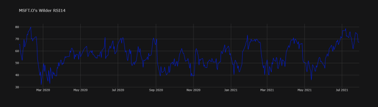
df = Refinitiv_RSI(ric_list=['MSFT.O'])
df.dropna()
| MSFT.O Close | MSFT.O's ln Return | MSFT.O's 1d Close | MSFT.O's Close 10D MA | MSFT.O's ln Return' 10D MA | MSFT.O's Ann. S.D. of 10D Roll. of ln Returns | MSFT.O's Close 30D MA | MSFT.O's ln Return' 30D MA | MSFT.O's Ann. S.D. of 30D Roll. of ln Returns | MSFT.O's Close 60D MA | MSFT.O's ln Return' 60D MA | MSFT.O's Ann. S.D. of 60D Roll. of ln Returns | MSFT.O's RSI14 | |
| 30/03/2020 | 160.23 | 0.067977 | 10.53 | 146.431 | 0.016823 | 0.996665 | 158.844 | -0.004855 | 1.170754 | 164.625167 | -0.000041 | 0.847859 | 52.673834 |
| 31/03/2020 | 157.71 | -0.015852 | -2.52 | 147.545 | 0.007325 | 0.919086 | 157.86 | -0.005719 | 1.170091 | 164.61 | -0.000096 | 0.848196 | 51.337963 |
| 01/04/2020 | 152.11 | -0.036154 | -5.6 | 148.716 | 0.008011 | 0.904883 | 156.687667 | -0.006933 | 1.174572 | 164.494667 | -0.000741 | 0.852745 | 48.400379 |
| 02/04/2020 | 155.26 | 0.020497 | 3.15 | 149.971 | 0.008429 | 0.906763 | 155.715667 | -0.005737 | 1.177938 | 164.456 | -0.000247 | 0.854052 | 50.129028 |
| 03/04/2020 | 153.83 | -0.009253 | -1.43 | 151.619 | 0.011332 | 0.862599 | 154.890333 | -0.004975 | 1.174237 | 164.351667 | -0.000665 | 0.853384 | 49.321227 |
| ... | ... | ... | ... | ... | ... | ... | ... | ... | ... | ... | ... | ... | ... |
| 23/07/2021 | 289.67 | 0.012261 | 3.53 | 281.613 | 0.004134 | 0.178585 | 272.2775 | 0.003958 | 0.161648 | 260.488917 | 0.002153 | 0.206477 | 75.427556 |
| 26/07/2021 | 289.05 | -0.002143 | -0.62 | 282.786 | 0.004143 | 0.178457 | 273.316167 | 0.003802 | 0.162964 | 261.097917 | 0.002252 | 0.205188 | 73.90081 |
| 27/07/2021 | 286.54 | -0.008722 | -2.51 | 283.342 | 0.001959 | 0.182599 | 274.2045 | 0.003254 | 0.167933 | 261.670583 | 0.002129 | 0.20677 | 67.908078 |
| 28/07/2021 | 286.22 | -0.001117 | -0.32 | 283.713 | 0.001305 | 0.181845 | 275.133167 | 0.003414 | 0.165493 | 262.24325 | 0.002131 | 0.206756 | 67.16034 |
| 29/07/2021 | 286.5 | 0.000978 | 0.28 | 284.26 | 0.001928 | 0.176626 | 276.103833 | 0.003573 | 0.163726 | 262.888417 | 0.002419 | 0.20163 | 67.497578 |
df["MSFT.O's RSI14"].dropna().iplot(title="MSFT.O's Wilder RSI14",
colors="#001EFF", theme="solar")