
The article demonstrates how to use Refinitiv Data Platform (RDP) Library for Python to retrieve historical data. Then, you can use the data for financial data science and plot the graph. In this article, we will show how to calculate some models i.e. log returns, correlation matrix, and linear OLS regression according to the data.
Introduction to the RDP Library for Python
Refinitiv Data Platform (RDP). is our cloud-enabled, open platform, that brings together content, analytics, customer, and third-party data distribution and management technology in one place. Hence, it would be ideal if a single library could be used to access that content which is in once place as well. That’s why Refinitiv Data Platform Libraries has been built. The libraries make simplify integration into all delivery platforms which are Refinitiv Workspace, or directly to RDP or Refinitiv Real-Time. The libraries provide a consistent API experience. You just learn once and apply across the wealth of Refinitiv content. The libraries reach the largest audience of developers possible from Citizen developers to seasoned professionals.
Python provides a large standard library including libraries to analyze data, create beautiful visualizations that reduce the length of code to be written significantly. It is also easy leaning. Hence, Python has been included in Refinitiv Data Platform Library. I will demonstrate how easy to use it to access historical data via RDP directly or Refinitiv Workspace.
The figure below is an architecture and layers from the RDP Libraries:
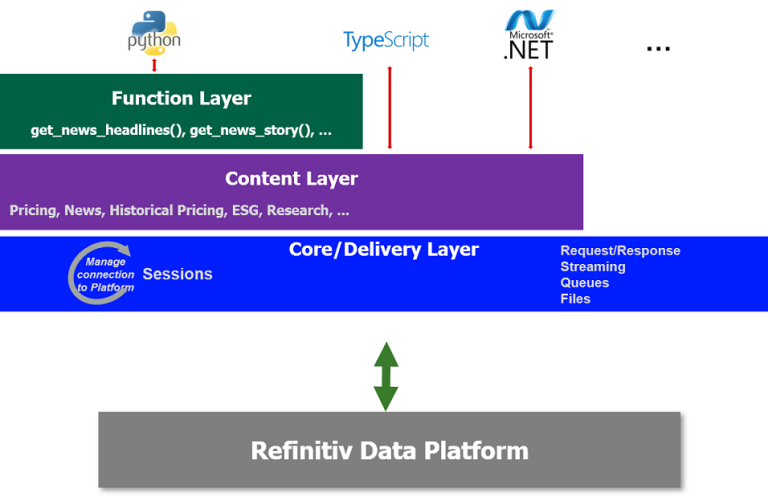
The RDP Library for Python is on the Function Layer which defines interfaces more suited to scripting languages such as Python. The goal of these interfaces is to allow researchers, data scientists, or the casual developer to rapidly prototype solutions within interactive environments such as Jupyter Notebooks. The Function layer provides simplistic data access in a single function call such as retrieving News Headlines and Stories, retrieving historical intraday, interday data, etc. Because this layer is built on top of the Content layer, it will benefit from convenient abstractions such as preparing data formats suitable for the specific programming language.
For more details, please refer to Refinitiv Data Platform Libraries - An Introduction.
Prerequisite
1. Access Credentials The RDP Library for Python allows the developer a consistent way to access content from multiple supporting access points e.g. Refinitiv Workspace, Refinitiv Data Platform/ERT in Cloud. The access credentials are required to retrieve content from RDP. Please refer to Access Credentials Quick Start for process and details on how to obtain the access credentials for each access point.
2. Python environment and package installer.
- Anaconda. It is the easiest way to perform Python data science and machine learning on Linux, Windows, and Mac OS X. It consists of Jupyter Notebook and the packages that we will require e.g. numpy, pandas. You can download and install Anaconda from here.
- cufflinks. When you import cufflinks, all Pandas data frames and series objects have a new method attached to them called .iplot(). Hence, the Pandas data frames can plot the graph. To install cufflinks:
- Open Anaconda Prompt
- Run the following command: pip install cufflinks
3. RDP Library for Python. To install the library:
- Open Anaconda Prompt:
- Run the following command: pip install refinitiv.dataplatform
4. If the content is accessed from the Refinitiv Workspace, make sure that you run version 1.8 or greater.
Implementation
1. Importing the libraries
import getpass
import refinitiv.dataplatform as rdp # the RDP library for Python
import pandas as pd
import numpy as np
import cufflinks as cf # to plot graph by pandas data frame
2. Opening a session
Depending on the access point your application uses to connect to RDP, it needs to create and open a platform or desktop session.
To access RDP directly. RDP username, password, and the application key are required.
RDP_USER = input("Enter RDP username: ")
RDP_PASSWORD = getpass.getpass('Enter RDP password:')
APP_KEY = getpass.getpass("Enter the app key: ")
We create and open a platform session with application key, RDP username and password to connect to RDP directly.
rdp.open_platform_session(
APP_KEY,
rdp.GrantPassword(
username = RDP_USER,
password = RDP_PASSWORD
)
)
Otherwise, to access RDP via Refinitiv Workspace. The application key is required.
APP_KEY = getpass.getpass("Enter the app key: ")
We create and open a desktop session with the application key.
rdp.open_desktop_session(APP_KEY)
3. Using RDP library for python
We call the get_historical_price_summaries(..) function to access year 2018 daily last price for each RIC. For more information of the get_historical_price_summaries(..) parameters, please refer to the get_historical_price_summaries Function Reference.
RICs = [".SPX",".VIX","IBM.N","GE"] # the list of RICs
s_date = "2018-01-02" # start date
e_date = "2018-12-30" # end date
#TBD - remove later pd.set_option('display.max_columns', None)
lastPriceField = "TRDPRC_1" # the last price field of these RICs
data = pd.DataFrame() # define data is a DataFrame
for aRIC in RICs: # request daily last price for each RIC
df= rdp.get_historical_price_summaries(aRIC,start=s_date,end=e_date,interval = rdp.Intervals.DAILY,fields=[lastPriceField])
if df is None: # check if there is any error
print("Error for RIC " + aRIC + ":" + str(rdp.get_last_status()['error'])) # print the error
else:
df[lastPriceField] = df[lastPriceField].astype(float) # convert string type to float
data[aRIC] = df[lastPriceField] # create the RIC's last price column
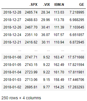
data # display daily last price of the RICs
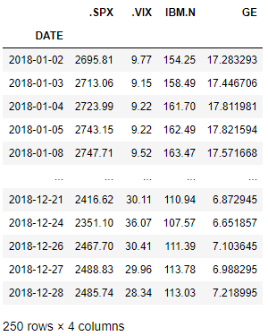
Next, we delete rows with NaN values and sort prices according to the DATE in ascending order.
data.dropna(inplace=True) # deletes rows with NaN values
data.index.names = ['DATE'] # set index name to be 'DATE'
data.sort_values(by=['DATE'], inplace=True, ascending=True) # sort prices according to the 'DATE' column in ascending order
data #display sorted prices
4.Calculating Financial Data Science models
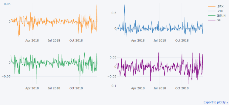
Log Returns [1]
Log Returns is the methods for calculating return and it assumes returns are compounded continuously rather than across sub-periods. It is calculated by taking the natural log of the ending value divided by the beginning value. (Using the LN on most calculators, or the =LN() function in Excel)
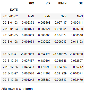
We calculate the Log Returns and display the result.
logReturns = np.log(data / data.shift(1)) # calculate the Log Returns
logReturns # display the result
To plot any graphs using Cufflinks, set the plotting mode to offline.
cf.set_config_file(offline=True)
Then, we plot the Log Return line graph of each RIC.
logReturns.iplot(kind='line', subplots=True)
Correlation Matrix [2]
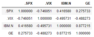
A Correlation Matrix is the Matrix of Correlation and dependence. Correlation and dependence is any statistical relationship, whether causal or not, between two random variables or bivariate data. In the broadest sense correlation is any statistical association, though it commonly refers to the degree to which a pair of variables are linearly related. Familiar examples of dependent phenomena include the correlation between the physical statures of parents and their offspring, and the correlation between the price of a good and the quantity the consumers are willing to purchase, as it is depicted in the so-called demand curve.
data.corr() # calculate the Correlation Matrix.
Then, we plot the Correlation Matrix graph of the RICs.
data.corr().iplot(kind='line')
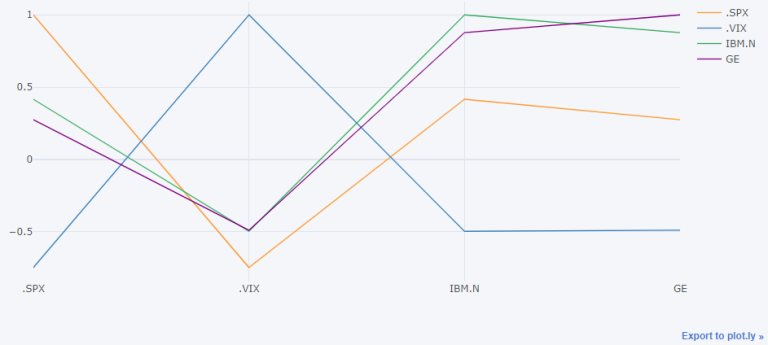
Correlations can be useful because sometime they will be able to indicate a predictive relationship that can be exploited in practice. For example, from the graph above, the prices of .SPX and IBM.N are in the analogous trend.
OLS Regression[3]
Ordinary least squares (OLS) regression is a statistical method of analysis that estimates the relationship between one or more independent variables and a dependent variable; the method estimates the relationship by minimizing the sum of the squares in the difference between the observed and predicted values of the dependent variable configured as a straight line. In this entry, OLS regression will be discussed in the context of a bivariate model, that is, a model in which there is only one independent variable ( X ) predicting a dependent variable ( Y ). However, the logic of OLS regression is easily extended to the multivariate model in which there are two or more independent variables.
For more details of the model, please refer to ORDINARY LEAST SQUARES REGRESSION (OLS)
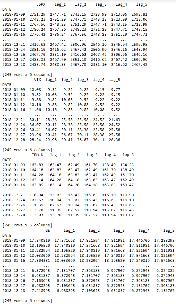
A. Preparing Lagged Data
The code that follows derives the lagged data for every single RIC. First, a function that adds columns with lagged data to a DataFrame object.
def add_lags(data, ric, lags):
cols = []
df = pd.DataFrame(data[ric]) #create data frame of the RIC
for lag in range(1, lags + 1):
col = 'lag_{}'.format(lag) # defines the column name
df[col] = df[ric].shift(lag) # creates the lagged data column
cols.append(col) # stores the column name
df.dropna(inplace=True) # gets rid of incomplete data rows
return df, cols
Next, the iterations over all RICs, using the add_lags function and storing the resulting DataFrame objects in a dictonary. Then, display the results.
dfs = {}
for ric in RICs:
df, cols = add_lags(data, ric, 5) # create the lagged data of a RIC
dfs[ric] = df # create the RIC's logged data column
print(dfs[ric]) # print the lagged data of the RIC
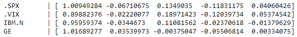
B. Implementing OLS Regression
The matrix consisting of the lagged data columns is used to "predict" the next day's value of the RIC via linear OLS regression.
regs = {}
for ric in RICs:
df = dfs[ric] # getting logged data of the RIC
reg = np.linalg.lstsq(df[cols], df[ric], rcond=-1)[0] # the OLS regression
regs[ric] = reg # storing the results
print('{:10} | {}'.format(ric, regs[ric])) # print the results
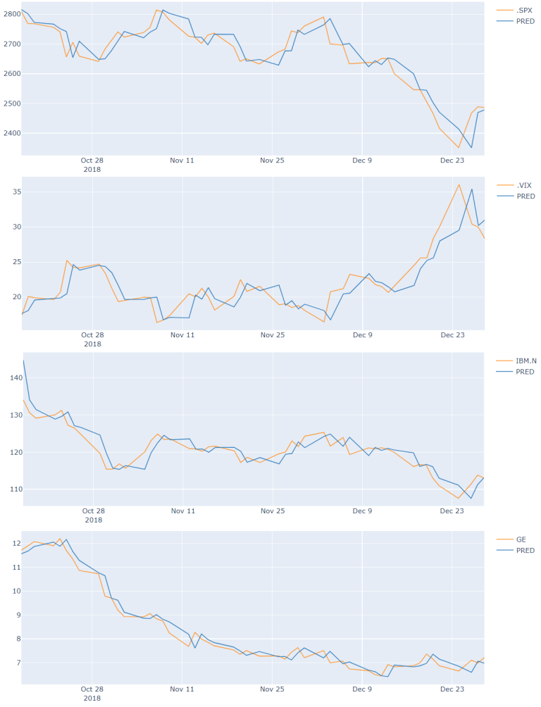
Comparing the original time series with the OLS predicted one
The predicted prices are almost the prices from the day before.
for ric in RICs:
res = pd.DataFrame(dfs[ric][ric]) # pick the data frame of the original time series
res['PRED'] = np.dot(dfs[ric][cols], regs[ric]) # creates the "prediction" values
layout1 = cf.Layout(height=450,width=1000)# Define a Layout with desired height and width
res.iloc[-50:].iplot(layout=layout1) # plot the graph
5. Close the session
rdp.close_session()
You can find the Jupyter Notebook of the complete source code on Article.RDPLibraries.Python.FinancialDataScience GitHub.
Troubleshooting
• Invalid username or password
2020-04-15 14:09:36,228 P[21140] [MainThread 21380] [Error 400 - access_denied] Invalid username or password.
Resolution: Make sure that RDP username and password are correct.
- Invalid Application Credential
2020-04-15 14:20:53,166 P[20540] [MainThread 20184] [Error 401 - invalid_client] Invalid Application Credential.
Resolution: Make sure that an Application Key is correct. You can check it from App key Generator.
- The universe is not found.
{'code': 'TS.Interday.UserRequestError.70005', 'message': 'The universe is not found.'}
Resolution: The RIC is not available in the system. The name of RIC may be incorrect. You should verify the RIC name or contact the data support team via Product Support of MyRefinitiv or use RIC Search Tool in order to find the correct RIC.
- The field is not found.
{'code': 'TS.Interday.UserRequestError.70007', 'message': 'The universe does not support the following fields: [<field>].'}
Resolution: The field is not provided by the RIC. The user can verify the available fields of the RIC by requesting historical data without fields parameter. For example, to find all fields of .SPX RIC, run the following source code:
df= rdp.get_historical_price_summaries(".SPX")
df
The example output:
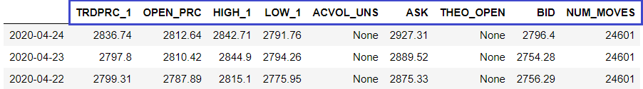
Then, you will see .SPX RIC provides 9 fields as shown above.
If you have any questions regarding the library usage, please post them on the Refinitiv Data Platform Libraries Q&A Forum. The Refinitiv Developer Community will be very pleased to help you.
get_historical_price_summaries Function Reference
The function provides historical data summaries for a RIC. The below is the declaration function and its parameters:
get_historical_price_summaries(universe, interval=None, start=None, end=None, adjustments=None, sessions=[], count=1, fields=[], closure=None)
Return: Historical pricing pandas data frame.
Parameters:
| Name | Type | Description |
|---|---|---|
| universe | string | Single RIC to retrieve historical data for |
| interval | refinitiv.dataplatform.Intervals | Data interval.
The default is DAILY. |
| start | string or datetime.datetime or datetime.timedelta |
The start of the query for historical pricing summaries. For interday summaries: String format is in ISO8601 with local date only e.g. '2018-01-02'. If the time is supplied, it will be ignored. For intraday summaries: String format is date and timestamp in ISO8601 with UTC only e.g. '2020-04-01T09:15:20Z'. Local time is not support. datetime.datetime is the datetime. datetime.timedelta is negative number of day relative to datetime.now(). Default is the earliest available. See more details on Start / End / Count handling section in Historical Pricing: Time Series Summary (bar), Events (T&S) Tutorial |
| end | string or datetime.datetime or datetime.timedelta |
The end of the query for historical pricing summaries. See more details on Start / End / Count handling section in Historical Pricing: Time Series Summary (bar), Events (T&S) Tutorial |
| adjustments | array[refinitiv.dataplatform.Adjustments | The list of adjustment types (comma delimiter) that tells the system whether to apply or not apply CORAX (Corporate Actions) events or exchange/manual corrections to historical time series data.
|
| sessions | array[refinitiv.dataplatform MarketSession] |
The list of market session classification (comma delimiter) that tells the system to return historical time series data based on the market session definition (market open/market close.
The supported values are:
|
| count | integer | It is the maximum number of data returned. If count is smaller than the total amount of data of the time range specified, some data (the oldest) will not be delivered. ee more details on Start / End / Count handling section in Historical Pricing: Time Series Summary (bar), Events (T&S) Tutorial |
| fields | array[string] | The comma-separated list of fields that are to be returned in the response. The fields value is case-sensitive, can be specified only with alphanumeric or underscore characters. If the parameter is empty or not specified, all available fields are returned. |
| closure | string | An identifier associated with an open data stream. Default: None |
Summary
In this article, we have quickly demonstrated how easy it is to retrieve historical data via RDP Libray for Python using the get_historical_price_summaries(..) function and calculate Log Returns, Correlation Matrix, and OLS Regression models using Cufflinks which makes financial data visualization convenient. This can be applied to any other models and calculations to serve more accurate or specific use cases.
References
"Log Return", in Log return definition and calculation in Excel. Retrieved Apr 23, 2020, from https://factorpad.com/fin/glossary/log-return.html
"Correlation and dependence", in Wikipedia. Retrieved Apr 23, 2020, from https://en.wikipedia.org/wiki/Correlation_and_dependence
"Ordinary Least Squares Regression" in Encyclopedia. Retrieved Apr 23, 2020, from https://www.encyclopedia.com/social-sciences/applied-and-social-sciences-magazines/ordinary-least-squares-regression
ORDINARY LEAST SQUARES REGRESSION (OLS), xlstat, https://www.xlstat.com/en/solutions/features/ordinary-least-squares-regression-ols
Refinitiv Data Platform Libraries, Refinitiv Developer Community, https://developers.refinitiv.com/refinitiv-data-platform/refinitiv-data-platform-libraries
Historical Pricing: Time Series Summary (bar), Events (T&S) Tutorial, Refinitiv Developer Community, https://developers.refinitiv.com/refinitiv-data-platform/refinitiv-data-platform-apis/learning?content=46324&type=learning_material_item
API Playground, https://apidocs.refinitiv.com/Apps/ApiDocs
Downloads