
Author:

In the previous article, we talked about applications of Quantum computing in Finance and saw how it can be used in Portfolio Optimization. In this article, we introduce options as financial instruments. We are going to propose the prevailing quantum approach in pricing European Options.
Let's have a short overview of what Qiskit Finance is, and what sub-modules it contains.

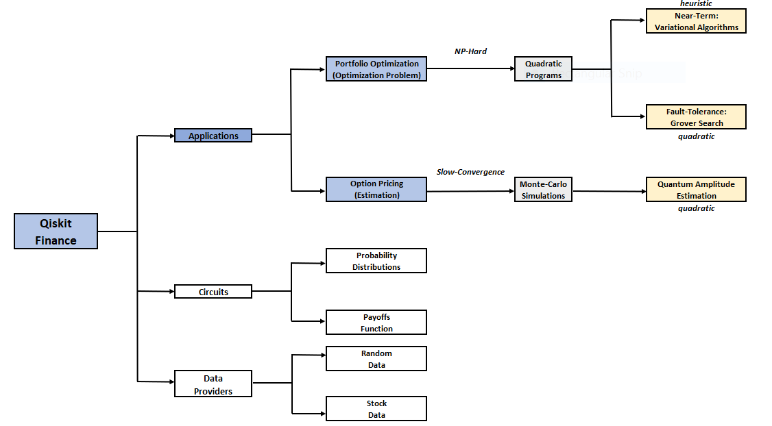
In the above diagram we can see that Qiskit Finance has two branches of applications:
- Portfolio Optimization
- Option Pricing
The package gives us the tools to solve optimization and option pricing problems such as the European Call Option or Fixed-Income Pricing. It also has sub modules containing circuits and tools to build the necessary quantum circuits to run these algorithms.
We can also see some modules for data providers that we can use to load random data or even load historical stock market data to test our algorithms. In this article we have extended the historical data loading module to allow it to load data from Eikon API.
Option Pricing Using Quantum Computers
Options, allow the buyer to exercise a certain amount of the underline stocks within a particular time frame. This helps reduce the risk taken from investment professionals. Some commonly used models to value options are the Black-Scholes Model, the Binomial Option Pricing, and Monte-Carlo Simulations. These methodologies have significant error margins error due to deriving their values from other assets.
The primary goal of option pricing theory is to calculate the probability that an option will be exercised or be In-The-Money (ITM), at expiration.
Commonly used variables used as input into these models include the underlying asset stock price, the exercise price, volatility, the interest rate and time to expiration, which is the number of days between the calculation date and the option’s exercise date. These mathematical models derive an option’s theoretical fair value and are quite integral in accurately pricing an option.
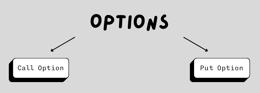
There are two type of options, Call Options, which give control to the option holder to buy stocks at a fixed value (strike price) within a certain time frame, and Put Options, that allow the option holder to sell stocks at fixed price within a certain time frame.
The simplest type is the European Options, which can be exercised at the time of maturity date only and can been modeled and calculated using the Black-Scholes model. The methodology assumes stock prices follow a Log Normal Distribution because asset prices cannot be negative.
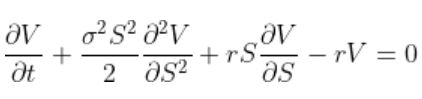
Black-Scholes Equation
Other assumptions made by the model are that there are no transaction costs or taxes, that the risk-free interest rate is constant for all maturities, that short selling of securities with use of proceeds is permitted, and that there are no arbitrage opportunities without risk. Indeed some of these assumptions do not hold true in real life scenarios.
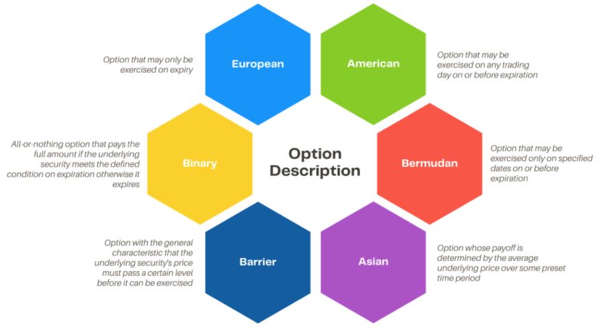
For the purposes of this prototype, we are going to focus on ‘vanilla’ European Options, the most fundamental type of an option contract. The majority of the exotic options are based on those and just introduce some kind of tweak to them. Time evolution of the price of a financial instrument can be modeled using a Wiener process called Geometric Brownian motion.
After this base introduction to options derivatives we can move on to how Quantum Computing can help us solve the option pricing problem.
Current Limitations
- As we are going through the early days of quantum computing it is expected that we will face a few limitations during the process, those mainly include:
- Quantum Systems still have a limited number of qubit available especially on public infrastructure layers.
- Fault-tolerant Quantum Systems to be built for quadratic speed up.
- More efficient ways to load classical data into quantum states and perform fast computations are still to be presented.
- Effective quantum error rate of the hardware is still somewhat high, however quantum error correction algorithms can be used to lower this.
Environment Setup & Package Installation
Assuming you already have anaconda installed and a python supported IDE in order to execute the below codes, you will need to install the following modules:
Qiskit Setup & Installation
Qiskit: An open-source SDK for working with quantum computers at the circuit level . It consists of algorithms, and application modules. For more info, visit here
Qiskit Finance: It contains uncertainty components for solving stock/securities problems, using translators for portfolio optimizations and data providers to ingest real or simulation data to finance experiments. For more info, visit here
Execute the below command in CMD to install Qiskit and it's components:
pip install qiskit qiskit-finance==0.2.1
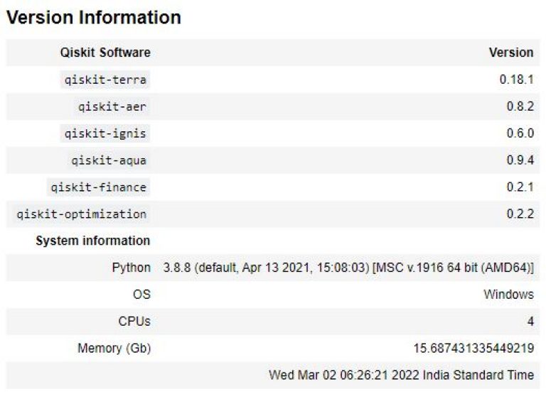
Check the version of Qiskit and it's installed components
import qiskit.tools.jupyter
%qiskit_version_table
[Optional] Setup token to run the experiment on a real device
If you would like to run this prototype on a real device, you need to setup your account first. You can get your API token from here.
Note: You can store your token in an environment variable, in a config file or use it directly, which is the least preferable approach in the command IBMQ.save_account('MY_API_TOKEN'). The command however will automatically save the token for the ongoing sessions.
from qiskit import IBMQ
IBMQ.save_account('MY_API_TOKEN', overwrite=True)
Eikon API Installation
Eikon API: It allows to access data directly from Eikon or Refinitiv Workspace using python. This allows data scientists and quants to prototype or productionize solutions. For more info, visit here.
Note: Eikon/Workspace Desktop application must be running for using Eiokn Data API.
Execute the below command in bash to install Eikon:
pip install eikon
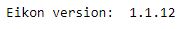
Check the version of Eikon API by using:
import eikon as ek
print("Eikon version: ", ek.__version__)
eikon_key = open("eikon.txt","r")
ek.set_app_key(str(eikon_key.read()))
eikon_key.close()
Other packages which needs to be installed, if not installed already, include pandas, matplotlib, seaborn
Importing Packages
import numpy as np
import pandas as pd
import datetime
import matplotlib.pyplot as plt
import seaborn as sns
import qiskit
from qiskit import Aer, QuantumCircuit
from qiskit_finance.data_providers._base_data_provider import BaseDataProvider
from qiskit.aqua import QuantumInstance
from qiskit.algorithms import IterativeAmplitudeEstimation
from qiskit_finance.circuit.library import EuropeanCallPricingObjective
from qiskit.circuit.library import LogNormalDistribution
from qiskit_finance.applications import EuropeanCallPricing
from qiskit_finance.applications.estimation import EuropeanCallDelta
Getting Data using Eikon API & Pre-Processing
Defining EikonDataProvider class for Loading Data as needed by Qiskit
We will inherit BaseDataProvider from data provider module of Qiskit Finance to extend it's functionality of getting data from Eikon API in desired format and make use of existing functions.
class EikonDataProvider(BaseDataProvider):
"""
The abstract base class for Eikon data_provider.
"""
def __init__(self, stocks_list, start_date, end_date):
'''
stocks -> List of interested assets
start -> start date to fetch historical data
end ->
'''
super().__init__()
self._stocks = stocks_list
self._start = start_date
self._end = end_date
self._data = []
self.stock_data = pd.DataFrame()
def run(self):
self._data = []
stocks_notfound = []
stock_data = ek.get_timeseries(self._stocks,
start_date=self._start,
end_date=self._end,
interval='daily',
corax='adjusted')
for ticker in self._stocks:
stock_value = stock_data['CLOSE']
self.stock_data[ticker] = stock_data['CLOSE']
if stock_value.dropna().empty:
stocks_notfound.append(ticker)
self._data.append(stock_value)
Initializing Required Parameters
# List of stocks
stock_list = ['FB.O']
# Start Date
start_date = datetime.datetime(2020,12,1)
# End Date
end_date = datetime.datetime(2021,12,1)
# Set number of equities to the number of stocks
num_assets = len(stock_list)
# Set the risk factor
risk_factor = 0.7
# Set budget
budget = 2
# Scaling of budget penalty term will be dependant on the number of assets
penalty = num_assets
Getting data from Eikon API using EikonDataProvider class
data = EikonDataProvider(stocks_list = stock_list, start_date=start_date, end_date=end_date)
data.run()
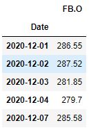
# Top 5 rows of data
df = data.stock_data
df.head()
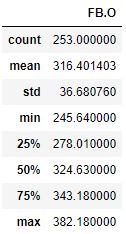
df.describe()
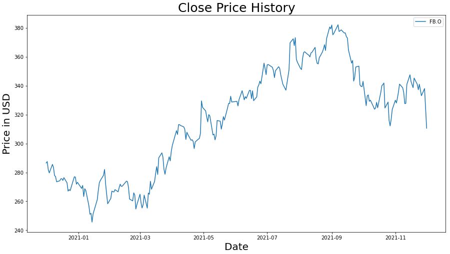
# Closing Price History
fig, ax = plt.subplots(figsize=(15, 8))
ax.plot(df)
plt.title('Close Price History',fontsize =25)
plt.xlabel('Date',fontsize =20)
plt.ylabel('Price in USD',fontsize = 20)
ax.legend(df.columns.values)
plt.show()
For the purposes of this article we are going to direct our attention towards the Qiskit Finance application module by IBM, more specifically we are going to look at the quantum computing approach for pricing European Call options. In the Qiskit tutorial we can look at the gradual construction of a circuit specific for European Call.
The Log Normal Distribution
A random variable X is said to have a lognormal distribution if its natural logarithm (ln X) is normally distributed. In case of a stock, we assume that the variable X represents the continuously compounded return of the stock price from time 0 to time T.
Some of the important characteristics of the lognormal distribution are:
- It has a lower bound of zero, i.e., a lognormal variable cannot take on negative values
- The distribution is skewed to the right, i.e., it has a long right tail
- If given two variables that follow the lognormal distribution, the product of the variables is also log-normally distributed.
A Lognormal model for stock prices can be defined as:
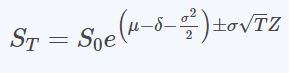
where,
μ = expected return on stock per year
σ = volatility of the stock price per year
T = time in years
δ = dividend yield (of a dividend paying stock)
ST = stock price at time T
S0 = stock price at time 0
Pre-defining few variables
strike_price = 315 # agreed upon strike price
T = 40 / 253 # 40 days to maturity
S = 310.6 # initial spot price
# vol = 0.4 # volatility of 40%
vol = df['FB.O'].pct_change().std()
r = 0.05 # annual interest rate of 4%
# resulting parameters for log-normal distribution
mu = ((r - 0.5 * vol**2) * T + np.log(S))
sigma = vol * np.sqrt(T)
mean = np.exp(mu + sigma**2/2)
variance = (np.exp(sigma**2) - 1) * np.exp(2*mu + sigma**2)
stddev = np.sqrt(variance)
# lowest and highest value considered for the spot price; in between, an equidistant discretization is considered.
low = np.maximum(0, mean - 3*stddev)
high = mean + 3*stddev
Call Option
sim = QuantumInstance(Aer.get_backend("aer_simulator"), shots=1000)
# number of qubits to represent the uncertainty
num_uncertainty_qubits = 5
distribution = LogNormalDistribution(num_uncertainty_qubits, mu=mu, sigma=sigma**2, bounds=(low, high))
european_call_pricing = EuropeanCallPricing(num_state_qubits=num_uncertainty_qubits,
strike_price=strike_price,
rescaling_factor=0.25, # approximation constant for payoff function
bounds=(low, high),
uncertainty_model=distribution)
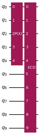
problem = european_call_pricing.to_estimation_problem()
problem.state_preparation.draw('mpl', style='iqx')
plt.show()
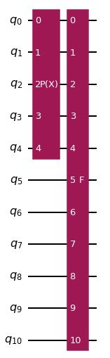
In this diagram, we can see the implementation of the Log-normal Distribution on the first layer and the Linear Amplitude Estimation function on the second layer. In both the European call and the European put implementations the core used algorithm is Iterative Amplitude Estimation. Crucially, this implementation does not rely on Quantum Phase Estimation, instead it relies only on selected Grover iterations. Essentially, we are interested in the probability of measuring ∣1⟩ in the last qubit.
epsilon = 0.01 # determines final accuracy
alpha = 0.05 # determines how certain we are of the result
ae = IterativeAmplitudeEstimation(epsilon, alpha=alpha, quantum_instance=sim)
result = ae.estimate(problem)
conf_int_result = np.array(result.confidence_interval_processed)
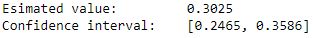
print("Esimated value: \t%.4f" % european_call_pricing.interpret(result))
print("Confidence interval: \t[%.4f, %.4f]" % tuple(conf_int_result))
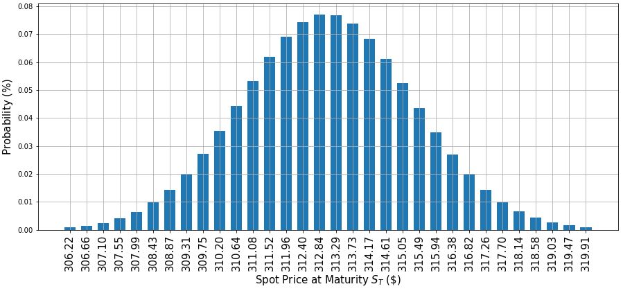
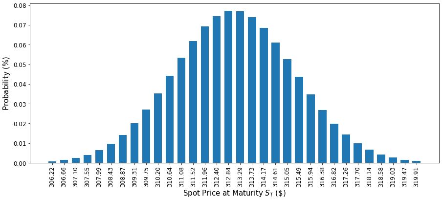
x = distribution.values
y = distribution.probabilities
plt.figure(figsize=(15,6))
plt.bar(x, y, width=0.3)
plt.xticks(x, size=15, rotation=90)
plt.yticks(size=10)
plt.grid()
plt.xlabel('Spot Price at Maturity $S_T$ (\$)', size=15)
plt.ylabel('Probability ($\%$)', size=15)
plt.show()
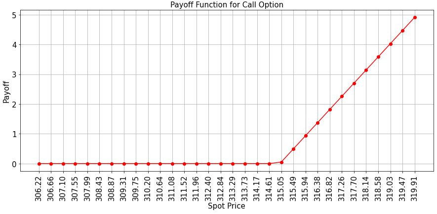
# plot exact payoff function (evaluated on the grid of the uncertainty model)
x = distribution.values
y = np.maximum(0, x - strike_price)
plt.figure(figsize=(15,6))
plt.plot(x, y, "ro-")
plt.grid()
plt.title("Payoff Function for Call Option", size=15)
plt.xlabel("Spot Price", size=15)
plt.ylabel("Payoff", size=15)
plt.xticks(x, size=15, rotation=90)
plt.yticks(size=15)
plt.show()
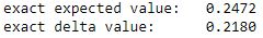
# evaluate exact expected value (normalized to the [0, 1] interval)
exact_value = np.dot(distribution.probabilities, y)
exact_delta = sum(distribution.probabilities[x >= strike_price])
print("exact expected value:\t%.4f" % exact_value)
print("exact delta value: \t%.4f" % exact_delta)
Evaluate Delta
The Delta is a bit simpler to evaluate than the expected payoff. Similarly, to the expected payoff, to calculate it, we use a comparator circuit and an ancilla qubit to identify the cases. However, since binary probabilistic problem, we can directly use the ancilla qubit as the objective qubit in amplitude estimation without any further approximation.
european_call_delta = EuropeanCallDelta(
num_state_qubits=num_uncertainty_qubits,
strike_price=strike_price,
bounds=(low, high),
uncertainty_model=distribution,
)
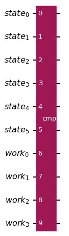
european_call_delta._objective.decompose().draw('mpl', style='iqx')
plt.show()
european_call_delta_circ = QuantumCircuit(european_call_delta._objective.num_qubits)
european_call_delta_circ.append(distribution, range(num_uncertainty_qubits))
european_call_delta_circ.append(
european_call_delta._objective, range(european_call_delta._objective.num_qubits)
)
european_call_delta_circ.draw('mpl', style='iqx')
plt.show()
# set target precision and confidence level
epsilon = 0.01
alpha = 0.05
problem = european_call_delta.to_estimation_problem()
# construct amplitude estimation
ae_delta = IterativeAmplitudeEstimation(epsilon, alpha=alpha, quantum_instance=sim)
result_delta = ae_delta.estimate(problem)
conf_int = np.array(result_delta.confidence_interval_processed)
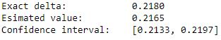
print("Exact delta: \t%.4f" % exact_delta)
print("Esimated value: \t%.4f" % european_call_delta.interpret(result_delta))
print("Confidence interval: \t[%.4f, %.4f]" % tuple(conf_int))
Put Option
put_distribution = LogNormalDistribution(num_uncertainty_qubits, mu=mu, sigma=sigma**2, bounds=(low, high))
put_european_call_pricing = EuropeanCallPricing(num_state_qubits=num_uncertainty_qubits,
strike_price=strike_price,
rescaling_factor=0.25, # approximation constant for payoff function
bounds=(low, high),
uncertainty_model=put_distribution)
put_problem = put_european_call_pricing.to_estimation_problem()
epsilon = 0.01 # determines final accuracy
alpha = 0.05 # determines how certain we are of the result
ae = IterativeAmplitudeEstimation(epsilon, alpha=alpha, quantum_instance=sim)
put_result = ae.estimate(put_problem)
put_conf_int_result = np.array(put_result.confidence_interval_processed)
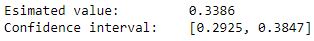
print("Esimated value: \t%.4f" % european_call_pricing.interpret(put_result))
print("Confidence interval: \t[%.4f, %.4f]" % tuple(put_conf_int_result))
x = put_distribution.values
y = put_distribution.probabilities
plt.figure(figsize=(15,6))
plt.bar(x, y, width=0.3)
plt.xticks(x, size=12, rotation=90)
plt.yticks(size=12)
plt.xlabel('Spot Price at Maturity $S_T$ (\$)', size=15)
plt.ylabel('Probability ($\%$)', size=15)
plt.show()
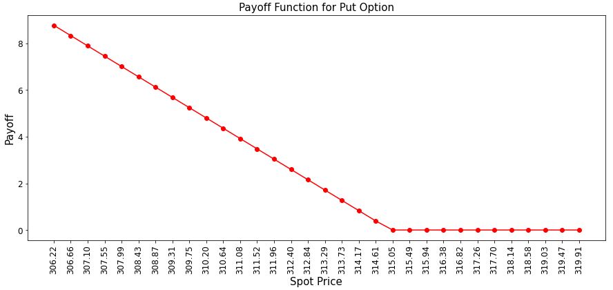
# plot exact payoff function (evaluated on the grid of the uncertainty model)
x = distribution.values
y = np.maximum(0, strike_price-x)
plt.figure(figsize=(15,6))
plt.plot(x, y, "ro-")
plt.title("Payoff Function for Put Option", size=15)
plt.xlabel("Spot Price", size=15)
plt.ylabel("Payoff", size=15)
plt.xticks(x, size=12, rotation=90)
plt.yticks(size=12)
plt.show()
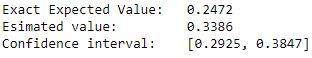
# evaluate exact expected value (normalized to the [0, 1] interval)
put_exact_value = np.dot(put_distribution.probabilities, y)
conf_int = np.array(put_result.confidence_interval_processed)
print("Exact Expected Value:\t%.4f" % exact_value)
print("Esimated value: \t%.4f" % european_call_delta.interpret(put_result))
print("Confidence interval: \t[%.4f, %.4f]" % tuple(conf_int))
Leveraging Qiskit Runtime
Due to in the limited number of qubits of the public layer of IBMQ systems, we will be using only 2 qubits to test it on real quantum computer. This somewhat lowers the accuracy of the solutions due to low quantization granularity however private layers can be used allowing up-to 50 qubit solutions now. You can find another notebook Option Pricing using Qiskit and Eikon Data API (Qiskit Runtime).ipynb for this.
Conclusion
We saw how to account for some of the more complex features present in european call options such as path-dependency with barriers and averages.
Future work may involve calculating the price derivatives with a quantum computer. Pricing options relies on Amplitude Estimation. The quantum approach delivers a quadratic speed-up compared to traditional Monte Carlo simulations. However, reaching a productionisation stage will most likely require the existence of a universal fault tolerant quantum computer.
Quantum computers are expected to have substantial impact in financial services, as they will eventually be able to solve certain problems considerably faster than the existing classical approaches.
Currently, it is a major challenge to determine when this impact will occur for each application. In fact, one of the most pressing challenges these days is to redesign quantum algorithms in a way that will considerably reduce the quantum hardware requirements while at the same time not deteriorate their proven performance superiority.
Advances in quantum algorithms together with better quantum hardware will continue to bring these applications closer to reality. I hope this article gives a good head-start in the exploration of the wonderful field of research on option pricing and quantum computing during the early days of this fast-evolving ecosystem.
References:
- European Call Option Pricing
- Portfolio Optimization using Qiskit and Eikon Data API
- TensorFlow Variational Quantum Neural Networks in Finance
- Option Pricing using Quantum Computers. Daniel J. Egger, Yue Sun, N.Stamatopoulos, C. Zoufal, R.Iten, Ning Shen, Stefan Woerner
- Quantuam Risk Analysis. Stefan Woerner , Daniel J. Egger
- Quantum Amplitude Amplification and Estimation. Gilles Brassard, Peter Høyer, Michele Mosca , Alan Tapp