


Introduction
Deep reinforcement learning (DRL) is one of the most recent Artificial Intelligence (AI) methodologies that has been applied cross-industry in very different use cases. In this Blueprint we will be exploring a DRL AI module that tries to detect the event of a flash crash. Building on the GAN Blueprint Flash Crash synthetic Data with Generative Adversarial Networks we will be using the features generated there, enhance the modelling space a bit more and try to train a DRL agent to understand the environment and give as an early detection signal of some possible abnormality within the market microstructure. We will be using Tensorforce as our Deep Reinforcement Learning framework a very recent module built from the Tensorforce team.
A primer on Deep Reinforcement Learning
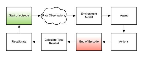
Deep Reinforcement Learning tries to imitate the way we us humans learn by experience and with the aid of experts around us. We live and evolve within our environment and as we observe the environment, we take decisions in it and we directly or indirectly receive rewards or suffer penalties as a result of our actions. Instinctively, we then tweak our behaviour trying to maximise our rewards and minimise our penalties. We continue exploring our environment and try to find new behavioural paths that will allow us to access new rewarding streams or avoid penalty paths. Oftentimes, this behaviour is fine-tuned by experts around us who are trying to help us achieve our goals. In such a way we continuously re-train and alter our behaviour. This is the exact process that DRL is trying to replicate. A digital twin of the environment is built, an agent is instantiated within the environment, an expert system defines the rewards and penalties stream and then the agent is allowed to explore the environment. As the agent takes decisions it is introduced with the appropriate rewards until it learns to optimally explore the environment and solve the problem that was digitally described. With proper modelling, it is possible to describe any type of problem and given an appropriate rewarding system and agent we should be able to solve the most complex of problems.
Modelling the market microstructure
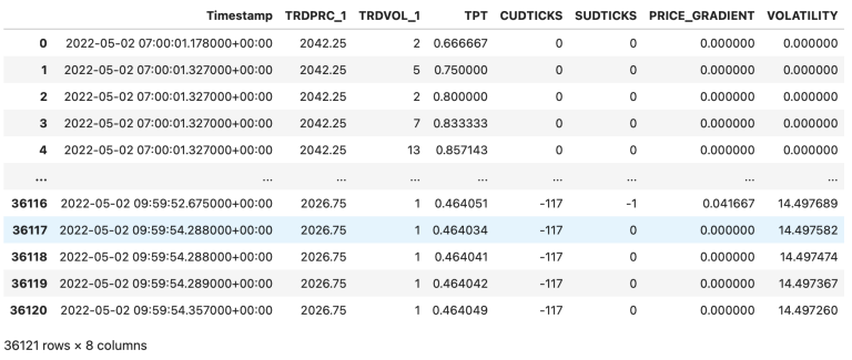
There are many features that can be engineered in an effort to model the market microstructure. We will be keeping the ones built in our Blueprint and engineer three more CUDTICK, SUDTICK and price volatility. The CUDTICK is the Cumulative Up-Down Ticks, whenever a trading up-tick is found in the raw data the counter increases by one and in the event of a down-tick it decreases by one. SUDTICK is the Sequential Up-Down Tick counter and counts the consecutive up or down ticks in the stream. The counter resets when there is a reversal in the raw data. Finally, volatility is the rolling standard deviation of price throughout a rolling observation period. We now have 8 features which we will be using to model the environment.
Building the Environment
The feature space is what mainly defines the environment and the flow of information during an episode. The main object that defines our environment also needs to define some of its dedicated functionalities. In the following code snippet, we can see how we can use the built-in Tensorforce class to instantiate our Exchange environment. We can see a few more functions introduced such as max_episode_timesteps() that is equal to the records count we have available and the reset() function that we use to bring the environment in its initial state. Here we are using it to rewind the iterators to the start of our dataset and the close() function that can be used for elegant termination of the code.
class ExchangeEnvironment(Environment):
def __init__(self):
super().__init__()
def states(self):
return dict(type='float', shape=(n,))
def actions(self):
return dict(type='int', num_values=d)
def max_episode_timesteps(self):
return super().max_episode_timesteps()
def close(self):
super().close()
def reset(self):
state = np.random.random(size=(n,))
return state
def execute(self, actions):
next_state = np.random.random(size=(n,))
terminal = False
reward = 0
return next_state, terminal, reward
The feature space schema
The feature space is what defines the view of our environment through each step within an episode. We use the function states() within an Environment object to define the types and shape of a dictionary that will be introduced to the agent at each step of the episode. In our case we define a dictionary of 8 floats that will be generated at each step.
def states(self):
state_dict = dict(type='float', shape=(7,))
return state_dict
Below we present the dataframe which includes first and last 5 observations of our feature space.
Building the agent
One of the critical entities of a DRL is the agent. It is the entity that lives in the environment we model and tries to explore it and solve the problem we have defined. Tensorforce provides us with numerous tools to define, pre-train, train, load and save multiple types of agent modules including the most popular DRL algorithms available:
· DQN: This agent is a value-based, offline reinforcement learning agent that trains a critic to estimate the future rewards. The optimal actions are derived from the action which maximizes the Q-value. DQN uses experience replay to learn from all past policies where transitions are randomly sampled to update the Q-value approximator.
· PPO: A policy-gradient method and unlike DQN, can work online without using a replay buffer. The algorithm optimizes the reward by estimating the policy gradient from the agent’s directions. This is an on-line method, where only the most recent transitions are used to update the policy.
· Actor – Critic: These methods combine both value-based and policy gradient methods where a critic network estimates the value of a state while the actor optimizes for the expected reward directly.
· Tensorforce: The most agile of the interfaces, allows to fully customise and build proprietary DRL agents.
One of the first design decisions we are faced with is the actions that are available to the agent within the environment. For this particular problem we allow the agent to take to decisions:
· The market microstructure looks normal
· The market microstructure seems abnormal
class Decision(enum.Enum):
NORMAL = 0
ABNORMAL = 1
This will allow us to build an alerting system to notify us should there exist any abnormality in the market and act accordingly. Coding this type of behaviour is pretty straight forward:
The next design decision is the initial hyper-parameter choice and values. A process that can be automatically optimised during training.
As the agent explores the environment it observes the state of each step and also the rewards it manages to accumulate by reaching that state given the decision vector it has followed up to that point. All this information for every step and episode can be found and accessed through the agent object. It is this insight that is used to alter the behaviour of the agent. Essentially, the agent explores all possible decision paths within the environment trying to find the one that will maximise its reward. It is not however unlikely that the agent will stop exploring as it finds a path that locally optimises the reward. It is the equivalent problem of local minima or maxima we frequently observe during neural network training. This is why it is important to randomly introduce some jitter in the path, using the appropriate hyper-parameters, to allow for further exploration and discovery of better decision paths should they exist.
class ExchangeAgent:
def __init__(self, environment: ExchangeEnvironment):
self.market_evaluation = Agent.create(
agent='dqn', environment=environment, batch_size=128, memory=len(y))
self.episode_actions = {}
In this Blueprint we use DQN agent since we wanted all observations to be included in the replay buffer in order for the agent to learn from all past experiences and make decisions to maximize the Q value. Replay memory is another important parameter that needs to be considered especially in DQN agents. Generally, the larger the memory, the less likely correlated samples will be sampled, and the training will be more stable. However, there is a trade-off using large memory as it requires a lot of RAM and it will slow down training. We therefore need to use a memory large enough to remember the whole state and yet small enough for better convergence. The size of all observations is used as a parameter value for replay memory in our model.
The agent actions
This is a function that defines the schema of the available actions to the agent conveniently called actions(). In this Blueprint we define a dictionary of two available actions.
def actions(self):
return {"DECISION": dict(type="int", num_values=2)}
The reward policy system
One of the most important structural elements of DRL is the reward policy which is what allows the DRL agent to learn from its behaviour. It is a very delicate part to calibrate and a very important factor in successfully training a DRL AI agent. The design and balancing of the reward system is a granular process that is fully proprietary depending on the problem at hand. Imbalancing of rewards and penalties can potentially prevent algorithms from converging to a solution.
During the first iterations of the design of the reward function we have built a reward variable which was calculated as the rolling standard deviation of the price and was reset as the flash crash periods starts. The idea behind resetting the calculation of volatility is to better capture the disruption of the market environment due to the crash, which requires the adjustment in the rewarding system. We use this reward variable to reward/penalize our agent while taking decisions about market normality/abnormality. Here is the function that builds the reward variable:
def generate_reward_feature(tick_data_frame):
data_before_fc = tick_data_frame.loc[pd.to_datetime(tick_data_frame.index) < pd.to_datetime(
flash_crash_event_starting_timestamp)]
data_before_fc['VOL'] = data_before_fc['TRDPRC_1'].expanding(
1).std().fillna(0)
data_after_fc = tick_data_frame.loc[pd.to_datetime(tick_data_frame.index) >= pd.to_datetime(
flash_crash_event_starting_timestamp)]
data_after_fc['VOL'] = data_after_fc['TRDPRC_1'].expanding(
1).std().fillna(0)
reward_variable = pd.concat([data_before_fc['VOL'], data_after_fc['VOL']])
return reward_variable
When it comes to the rewarding policy of the RL agent, it follows the concepts below:
- Early termination: A heavy penalty in case of early termination caused by early stopping criteria 1 & 2 introduced in the respective section below. This penalty is applied only if early termination is activated.
- Before the crash: A positive reward equal to the current state reward variable in case the agent is diagnosing a normal market state and 0 otherwise.
- During the crash: A penalty (negative reward) equal to the current state reward variable in case the agent is diagnosing a normal market state and 0 otherwise.
- After the crash: A penalty (negative reward) equal to the 3 times of the current state reward variable in case the agent is diagnosing an abnormal market state and 0 otherwise.
The code snippet below presents the code for modeling the described reward function.
def calculate_reward(self, reward_val, timestamp, decision, terminal):
if terminal is True and pd.to_datetime(timestamp) < pd.to_datetime(flash_crash_event_ending_timestamp):
reward = -200
else:
if pd.to_datetime(timestamp) < pd.to_datetime(flash_crash_event_starting_timestamp):
if decision == Decision.NORMAL.value:
reward = reward_val
else:
reward = 0
elif pd.to_datetime(flash_crash_event_starting_timestamp) <= pd.to_datetime(timestamp) <= \
pd.to_datetime(flash_crash_event_ending_timestamp):
if decision == Decision.NORMAL.value:
reward = -reward_val
else:
reward = 0
elif pd.to_datetime(timestamp) > pd.to_datetime(flash_crash_event_ending_timestamp):
if decision == Decision.ABNORMAL.value:
reward = -3*reward_val
else:
reward = 0
return reward
Execution policy
The execute() function is the main function that gets triggered at each episode. The main function should perform three actions at minimum. Check for early stopping conditions, calculate the current state reward and define the next state of the environment.
def execute(self, all_decisions, actions):
timestamp = self.environment_observations.index[self.state_iterator]
self.state_iterator += 1
reward_val = self.reward_var.iloc[self.state_iterator]
next_state = self.environment_observations.iloc[self.state_iterator]
terminal = self.check_terminal_criteria(
actions, all_decisions, timestamp, early_terminate=False)
reward = self.calculate_reward(reward_val,
timestamp, actions['DECISION'], terminal)
return next_state, terminal, reward
The episode stopping conditions
For various reasons, during training, we might want to stop an episode before it plays the full step count. Perhaps the performance is deteriorating and there is no need for the agent to continue exploring in the same directions or a critical constraint has been triggered. In our Blueprint we keep it simple and just add a sample constraint.
def check_terminal_criteria(self, actions, all_decisions, timestamp, early_terminate=False):
terminate = False
cutoff_timestamp = '2022-05-02 07:58:20.119000+00:00'
if early_terminate:
if pd.to_datetime(timestamp) < pd.to_datetime(flash_crash_event_starting_timestamp) and \
actions['DECISION'] == 1:
terminate = True
elif pd.to_datetime(timestamp) > pd.to_datetime(cutoff_timestamp) and \
sum(all_decisions) == 0:
terminate = True
if self.state_iterator == self.no_states - 1:
terminate = True
return terminate
Training the agent
Now that we have modelled the environment and have defined our DRL agent, training the agent is a process of exposing it into the environment and allow it to freely explore by taking decisions in it. We define two new terms in the context of DRL the episode and step. An episode is a full pass of the agent within the feature space (essentially, we will be replaying our tick data space within each episode). A step is the equivalent of an epoch within an episode. It is important to keep track of various statistics during DRL training to help us understand the behaviour of the agent as it tries to navigate the environment. This can provide a lot of intuition and help us tweak and optimise the design. Two of the most important parameters to keep track of is the reward vector as well as the decision vector.
Once we identify the optimal episode, we need to be able to save the agent that was performing in the environment so that it can be used in production. Tensorforce allows us to easily save and retrieve agent models through its built-in interface. It is important to save every trained agent as we replay the episodes in order to retrieve the optimal model after training.
def execute_episode_batch(environment: ExchangeEnvironment, agent: ExchangeAgent, episodes):
for i in range(episodes):
episode_length = 0
state_vector = environment.reset()
terminate = False
while not terminate:
episode_length += 1
actions = agent.market_evaluation.act(states=state_vector)
state_vector, terminate, reward = environment.execute(all_decisions,
actions=actions)
agent.market_evaluation.observe(
terminal=terminate, reward=reward)
all_decisions.append(actions['DECISION'])
Results on the OMX event
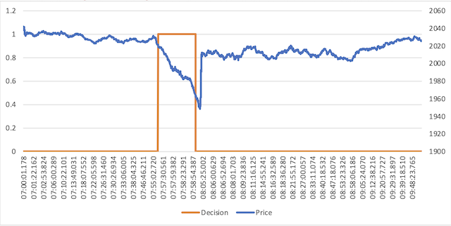
The RL agent has been trained on the recent flash crash event that happened on May 2, 2022 during which European stock markets crashed for about 5 minutes. Particularly, the Swedish OMXS30 index dropped 6.8%, the Norwegian OBX 4.1%, the Danish OMXC25 -6.7% and the Finnish OMXH25 -7.5%.
We used approximately 40,000 data ticks on the crash date from the Swedish OMXS30 index, and, following the methodology described in the respective sections above, we have trained a RL agent which after a couple of hundred episodes of training showed promising results generating the decisions seen in the following graph, where a decision of 0 depicts normal market behaviour and a decision of 1 abnormal market behaviour:
Conclusions
In this Blueprint we have presented a primer on Deep Reinforcement Learning architectures. We have implemented the main components including the environment, the agent, the rewarding policies, as well as an initial training process. The main purpose of the RL agent was to predict if the market microstructure is residing in a normal state or not, hoping that this would allow the AI to identify if there is an imminent instability in the market such as a flash crash. To architect the system, we have used a day’s worth of tick data from the Swedish OMXS30 index and engineered 8 features, including cumulative and subsequential tick directions, price gradient and volatility. Furthermore, we have implemented a DQN agent which was introduced to a proprietary rewarding system as it was observing the environment and making decisions in it. After numerous episodes of training, we have received promising results showing that this Blueprint could prove a useful wireframe for further research in the field. Furthermore, this RL model can be used to detect other market microstructure change scenarios.