This article builds on our TensorFlow Variational Quantum Neural Networks in Finance where we have used Qiskit to inject a simple Quantum layer within a Tensorflow deep neural network structure. Here, within the same DNN structure, we will be injecting a more complex layer structure that is implementing a Quantum Fourier Transform (QFT) on its inputs. This will allow us to explore how such an integration can be implemented and the effects this more complex transformation layer has on the DNN performance. We will explore how we can implement a dynamic QFT layer in Q#, able to scale up to a variable number of Qubits, and how such a layer can be simulated locally using the Microsoft.Quantum namespace or executed on Azure Quantum. Finally using the Refinitiv Data Libraries we will be testing the structure by generating a simple trading signal on historical stock price data.
Getting ready to implement the Quantum Fourier Transform in Q#
For the purposes of this article, we will be implementing the QFT in Q#. We will aim to implement the quantum circuit that executes the transformation using a dynamic number of qubits that is only constrained from the current quantum hardware qubit availability.
Let’s start by building our development environment. All the examples were implemented using VSCode with the pylance and Quantum Development Kit extensions installed. It is good practice to start a new anaconda environment that can be used to install all the necessary packages including:
Also, we will need to install the following:
Once the Azure CLI package. VSCode should download and install IQ# Server the first time it will execute your Q# program. If this does not happen, we need to install the package manually in the anaconda environment. Once all the installations are ready, we can start an anaconda prompt and run the command code to start VSCode in the correct environment, then navigate to the terminal and run:
python -c “import qsharp”
To activate and load the package cache in memory. For the tensorflow integrations we will also need to download the QuantumDense library from this article repository.
Finally, to test execution on Azure Quantum we will need an Azure subscription and a Quantum workspace at your preferred location.
Discrete Fourier Transforms
In the field of Digital Signal Processing (DSP) the Discrete Fourier Transform (DFT) is one of the main tools used to manipulate data signals. It is used to transform a signal from its time domain to a frequency domain allowing us to decompose any time series into a sum of sinusoidal functions. In math terms if we had a f(x) signal, then we would define its DFT as:
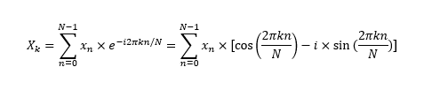
Where: N is the number of samples, n is our current sample, k is the current frequency, x(n) is the sine value at sample n and x(k) is the DFT which includes information on amplitude and phase. Using such a process, any signal can be transformed using DFT into a collection of amplitudes and phases of the individual sinusoidal signals. The amplitude and phase of the signal can be calculated as:
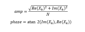
Furthermore, applying the inverse process to the amplitude and phase frequency space, we can reconstruct the original signal. The DFT process has a lot of applications in many industries including finance where some of its more important use cases include signal denoising and options pricing.
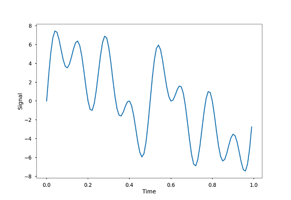
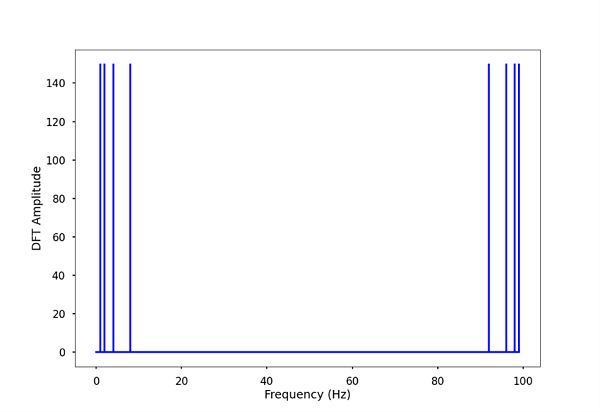
Let’s write a simple example to understand the concept and then apply it to a price time series. In this example we will construct a time series from four sinusoidal waves at 1, 2, 4 and 8 Hz, and then apply the DFT formulas to transform it to frequency space:
import matplotlib.pyplot as plt
import numpy as np
plt.style.use('seaborn-poster')
sampling_rate = 100.0
sampling_interval = 1.0 / sampling_rate
t = np.arange(0, 1, sampling_interval)
frequency = 1 # Hz
x = 3 * np.sin(2 * np.pi * frequency * t)
frequency = 2 # Hz
x += 3 * np.sin(2 * np.pi * frequency * t)
frequency = 4 # Hz
x += 3 * np.sin(2 * np.pi * frequency * t)
frequency = 8 # Hz
x += 3 * np.sin(2 * np.pi * frequency * t)
plt.plot(t, x)
plt.show()
We can now write the DFT function and apply it on this signal to analyse it:
def DFT(x):
N = len(x)
n = np.arange(N)
k = n.reshape((N, 1))
e = np.exp(-2j * np.pi * k * n / N)
X = np.dot(e, x)
return X
X = DFT(x)
N = len(x)
n = np.arange(N)
T = N / sampling_rate
frequency = n / T
plt.stem(frequency, abs(X), 'b', markerfmt=" ", basefmt="-b")
plt.xlabel("Frequency (Hz)")
plt.ylabel("DFT Amplitude")
plt.show()
In the resulting image we can see that the DFT correctly analysed the time series into its four constituents. We need to take into account only the left hand side of this mirrored graph.
Testing the correct implementation of the DFT in Q# and Jupyter
Once the environment is initialised, we can start a powershell and activate it. After that, we should be able to start a jupyter notebook with the Q# extensions enabled and write a Q# program. Furthermore, the environment and all the tools we installed, provide us with very interesting new Quantum related functionality within our jupyter notebook. Let’s now write and test the Q# code that implements the Quantum Fourier Transform:
First, we need to include the appropriate .Net libraries:
open Microsoft.Quantum.Canon;
open Microsoft.Quantum.Intrinsic;
open Microsoft.Quantum.Measurement;
open Microsoft.Quantum.Math;
open Microsoft.Quantum.Convert;
open Microsoft.Quantum.Arrays;
open Microsoft.Quantum.Diagnostics;
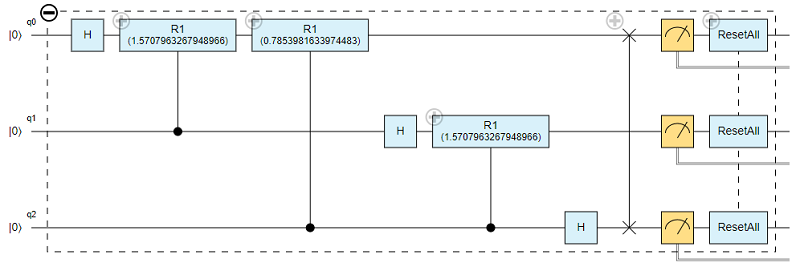
A callable in Q# can be either an operation that can be executed in a simulator or on Azure Quantum hardware or a functor. Let’s write a Quantum operation that implements the Fourier transform. We will also use the DumpMachine() function to log the quantum register state in order to diagnose and debug the execution of the circuit.
operation QuantumFourierTransform(n: Int) :Result[] {
mutable output = [Zero, size=n];
mutable stage_degree_fraction = 2.0;
use quantum_register = Qubit[n];
for i in 0 .. Length(quantum_register) - 1 {
H(quantum_register[i]);
for k in i+1 .. Length(quantum_register) - 1 {
for fr in 0 .. (k-i-2){
set stage_degree_fraction = stage_degree_fraction * 2.0;
}
Controlled R1([quantum_register[k]], (PI()/stage_degree_fraction, quantum_register[i]));
set stage_degree_fraction = 2.0;
}
}
for i in 0 .. n/2 - 1 {
SWAP(quantum_register[i], quantum_register[n-1]);
}
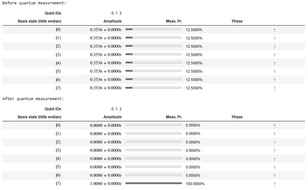
Message("Before quantum measurement:");
DumpMachine();
for i in IndexRange(quantum_register){
set output w/= i <- M(quantum_register[i]);
}
Message("After quantum measurement:");
DumpMachine();
ResetAll(quantum_register);
return output;
}
Let’s use the magic command %trace to draw the corresponding Quantum Circuit:
We can also use the %simulate command to execute the circuit in the local full state simulator.
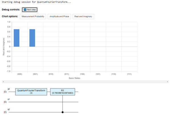
A very interesting functionality is the %debug magic command which allows us to check all the interim stages of the qubit as each gate transformation is applied to the register:
We can finally submit the circuit for simulation using any of the available Azure Quantum endpoints. The following code uses the ionq simulator to push the circuit on our Azure quantum workspace. The resourceId and location of our workspace need to be passed as parameters:
%azure.connect resourceId=”" location=""
%azure.target ionq.simulator
%azure.execute QuantumFourierTransform n=2
Further testing the integration of Q# and python
Now that we have the correct circuit built in Q# let’s turn to VSCode and see if we can call an operation written in Q# from a python project. The python application that calls the Q# operation is called the host. Here is a small operation setting a quantum register into superposition with custom theta and phase. The code is written in a .qs file which resides in the same folder as the python host application:
operation SuperpositionQubit(theta : Double, phase : Double) : Result {
use q = Qubit();
Rx(theta, q);
Ry(phase, q);
return M(q);
}
Turning to our host python application, we need to import qsharp first which will allow us to use packages written in Q# within our host:
import qsharp
from QuantumSpace import QuantumRegister, QuantumFourierTransform, SuperpositionQubit
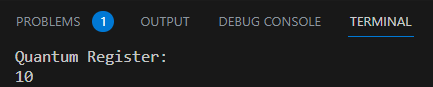
print('Superposition qubit:')
print(SuperpositionQubit.simulate(theta=0.5, phase=0.5))
If the installation and integration is working correctly then we will see a message that .Net is preparing the Q# environment and then a simple 2-digit binary result. This is the result returned from our local quantum simulator. There is a chance that we will also receive an error message about an ignored exception that was thrown from the python interpreter as the QuantumSpace module is not known to the environment and the integration is achieved through IQ# server. The exception itself does not affect the execution of the program.
Integrating Tensorflow with the QFT layer
Now that we have a working integration between Q# and python and a Quantum Fourier Transform circuit it is time to write the Discrete Fourier Transform and integrate that with the rest of the Tensorflow structure. We can copy the code from the Q# Notebook in the VSCode Q# solution omitting the DumpMachine sections. We also need to implement a few more changes at the start of the operation, as we will be adding theta and phase training in the structure. We remove the Hadamard gate and add two Pauli Rotation gates along with the relevant parameters.
operation QuantumFourierTransform(n: Int, thetas : Double[], phases : Double[]) :Result[] {
mutable output = [Zero, size=n];
mutable stage_degree_fraction = 2.0;
use quantum_register = Qubit[n];
for i in 0 .. Length(quantum_register) - 1 {
Rx(thetas[i], quantum_register[i]);
Ry(phases[i], quantum_register[i]);
...
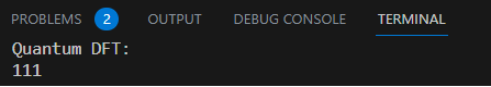
We can now call the Q# operation through our python host.
import qsharp
from QuantumSpace import QuantumFourierTransform
print('Quantum DFT:')
print(''.join(map(str, QuantumFourierTransform.simulate(n=3, thetas=[0.5, 0.5, 0.5], phases=[0.5, 0.5, 0.5]))))
If the execution was successful, the output will look like:
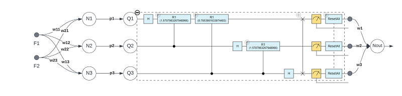
The layer is working and is callable through python so we can now continue to incorporate the necessary changes within the QuantumDense.py module. As expected, this is a case of a proprietary layer that is injected in a Tensorflow Sequential neural network structure, during the forward phase, the previous layers will drive the QFT layer. The QFT layer module inherits from the tensorflow.keras.layers.Layer overriding all necessary functionality to implement a QFT circuit that is able to apply a Fourier transformation on the input it receives. Because the layer inherits from a Tensorflow Layer class, it can be used as any of the available layers in the framework. The next schematic shows how a 3-Qubit QFT layer may be connected to a prior classical three neuron layer receiving two features as input. The transformed output of the QFT layer is a continuous vector with as many constituents as the qubits used during the Fourier transform. This output can then be used as a driver to a following layer, in this case we use it before a Dense layer for regression.
The following code implements a hybrid Quantum NN structure that is fully dynamic and can be parameterised to receive any number of inputs and have any structure that may be appropriate for the problem at hand. Here we instantiate a 3 layered Quantum Neural Network with the following layers:
· A Dense neural layer with a relu activation function
· Our Quantum Fourier Transform layer
· A single neuron Dense layer acting as a regression layer for our use case
class VQNNModel(tf.keras.Model):
def __init__(self):
super(VQNNModel, self).__init__(name='VQNN')
self.driver_layer = tf.keras.layers.Dense(3, activation='relu')
self.quantum_layer = QFTLayer(2)
self.output_layer = tf.keras.layers.Dense(1)
def call(self, input_tensor):
try:
x = self.driver_layer(input_tensor, training=True)
x = self.quantum_layer(x, training=True)
x = tf.nn.relu(x)
x = self.output_layer(x, training=True)
except QuantumCircuitModuleException as qex:
print(qex)
return x
We can now turn to the actual integration of the Q# DFT layer and its implementation. First we need a Quantum layer that derives from Layer:
class QFTLayer(Layer):
def __init__(self, qubits=3, execute_on_AzureQ=False):
super(QFTLayer, self).__init__()
self.qubits = qubits
self.tensor_history = []
self.execute_on_AzureQ = execute_on_AzureQ
self.circuit = QuantumCircuitModule(self.qubits)
def build(self, input_shape):
kernel_p_initialisation = tf.random_normal_initializer()
self.kernel_p = tf.Variable(name="kernel_p",
initial_value=kernel_p_initialisation(shape=(input_shape[-1],
self.qubits),
dtype='float32'),
trainable=True)
kernel_phi_initialisation = tf.zeros_initializer()
self.kernel_phi = tf.Variable(name="kernel_phi",
initial_value=kernel_phi_initialisation(shape=(self.qubits,),
dtype='float32'),
trainable=True)
def call(self, inputs):
try:
output = tf.matmul(inputs, self.kernel_p)
quantum_register_output = self.circuit.quantum_execute(tf.reshape(output, [1, self.qubits]), self.kernel_phi)
quantum_register_output = tf.reshape(tf.convert_to_tensor(quantum_register_output), (1, 1, self.qubits))
output += (quantum_register_output - output)
except QuantumCircuitModuleException as qex:
raise qex
return output
Notice that the QFTLayer class implements the neccessary functions build() and call() as well as the trainable layer parameters p and phi. Finally, we implement a helper class that defines the implementation of the layer core as well as its training process:
class QuantumCircuitModule:
def __init__(self, qubits=3):
self.qubit_num = qubits
self.probabilities = tf.constant([[0.5] * self.qubit_num])
self.phase_probabilities = tf.constant([1] * self.qubit_num)
self.thetas = []
self.phis = []
def p_to_angle(self, p):
try:
angle = 2 * np.arccos(np.sqrt(p))
except Exception as e:
raise QuantumCircuitModuleException(
QuantumCircuitModuleExceptionData(str({f"""'timestamp': '{datetime.datetime.now().
strftime("%m/%d/%Y, %H:%M:%S")}',
'function': 'p_to_angle',
'message': '{e.message}'"""})))
return angle
def superposition_qubits(self, probabilities: tf.Tensor, phases: tf.Tensor):
try:
reshaped_probabilities = tf.reshape(probabilities, [self.qubit_num])
reshaped_phases = tf.reshape(phases, [self.qubit_num])
static_probabilities = tf.get_static_value(reshaped_probabilities[:])
static_phases = tf.get_static_value(reshaped_phases[:])
self.thetas = []
self.phis = []
for ix, p in enumerate(static_probabilities):
p = np.abs(p)
theta = self.p_to_angle(p)
phi = self.p_to_angle(static_phases[ix])
self.thetas.append(theta)
self.phis.append(phi)
except Exception as e:
raise QuantumCircuitModuleException(
QuantumCircuitModuleExceptionData(str({f"""'timestamp': '{datetime.datetime.now().
strftime("%m/%d/%Y, %H:%M:%S")}',
'function': 'superposition_qubits',
'message': '{e.message}'"""})))
Most of this code has been explained in our previous article TensorFlow Variational Quantum Neural Networks in Finance, however there are a few changes to support this new integration with Q#. The main change is in quantum_execute and the way inputs and outputs flow within the Q# layer:
def quantum_execute(self, probabilities, phases):
try:
self.superposition_qubits(probabilities, phases)
circuit_result = ''.join(map(str, QuantumFourierTransform.simulate(n=self.qubit_num, thetas=self.thetas, phases=self.phis)))
qubits_results = [float(x) for x in list(circuit_result)]
qubit_tensor_results = tf.convert_to_tensor(qubits_results, dtype=tf.float32)
except Exception as e:
raise QuantumCircuitModuleException(
QuantumCircuitModuleExceptionData(str({f"""'timestamp': '{datetime.datetime.now().
strftime("%m/%d/%Y, %H:%M:%S")}',
'function': 'quantum_execute',
'message': '{e.message}'"""})))
return qubit_tensor_results
The use case and new results
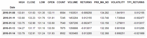
As a quick reminder of the use case, we will use daily price data for a single RIC and engineer a few features to generate a simple trading signal. The main code of the use case remains the same. Here is a dataframe after generating features RETURNS, PRX_MA_ND the moving average of price last 5 days and VOLATILITY using the raw dataset:
Thereafter, we set the next day up or down tick of returns TP1_RET_UDT as the target variable for our model, effectively turning this into a classification problem. We also set aside 2021 data for forward trading tests. The rest of the transformations remain the same. Furthermore, the code for training, testing and evaluating the new structure remains the same. And the results are again plotted using a custom matplotlib plot:
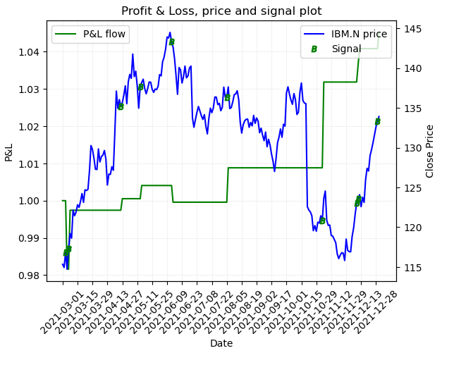
We can see that the new VQNN structure with the DFT layer implemented is generating a less aggressive signal than the original one making roughly a 43% profit over a period of 175 days’ worth of forward trading in 2021. This again is a very loose assumption as no other factors are considered within the backtesting process including TCA, maintenance, and post trading analytics. However, the main purpose of this article is to showcase how we can write a prototype ingesting Refinitiv data within the ecosystem of Azure Quantum using the Q# language to write a complex Discrete Fourier Transform neural layer. We also utilise the TensorFlow ecosystem for AI and integrate our Q# with that by connecting python and Q#. The process itself is again evidence of the possible integrations of quantum and classical computing.
Conclusions and future work
This article showcases how we can implement a Discrete Fourier Transform Quantum Neural Layer using Q# and inject it into a Variational Quantum Neural Network implemented in Tensorflow. Leveraging upon the rich data ecosystem provided by Refinitv, we have used the hybrid quantum – classical structure to implement a simple trading signal. In the future, we will further explore the concept, by trying the infrastructure in other data scenarios. This new DFT QuantumDense layer can participate both in regression and classification AI structures. The new layer is executed on the available Microsoft Quantum simulators locally and can also be run on Azure Quantum on its own. As our next steps we are looking to achieve a full classical - hybrid on-the-cloud implementation utilising the Microsoft Azure ecosystem of services. Such an experiment on its own can produce valuable insight in the Quantum space.
If you would like to reach out with any questions regarding this article, we would be happy to address those in our Developer Community Q&A Forum.
- Register or Log in to applaud this article
- Let the author know how much this article helped you