
Webinar
Introduction
Since Tinbergen (1933)'s modelling work on business cycles post World War I, many econometric methods were developed with the aim of constructing ever better economic and financial forecasts. The subject evolved through statistical linear and non-linear relationships with Autoregressive (AR) (Yule (1927)), Moving Average (MA) (N. and Wold (1939)), Autoregressive Moving Average (ARMA) (Whittle (1951)), Autoregressive Conditional Heteroskedasticity (ARCH) (Engle (1982)), Generalized ARCH (GARCH) (Bollerslev (1986)), Exponential GARCH (EGARCH) (Nelson (1991)), threshold nonlinear ARMA (Tong (1990)), and Glosten- Jagannathan-Runkle GARCH (GJR-GARCH) (Glosten, Jagannathan, and Runkle (1993))) models amongst others.
Stylized Facts of Financial Return (SFFR)
These models’ uses in financial time-series analysis have grown to become staple tools in academia; but many came upon what are now well established asset return forecasting challenges: Stylized Facts of Financial Return (SFFR) - a set of properties found in most asset return datasets (Booth and Gurun (2004); Harrison (1998); Mitchell, Brown, and Easton (2002)). Many SFFR exist, but only a few are of interest in this instance: asset returns' (i) non-Gaussian distribution (unconditional leptokurtosis/excess-kurtosis and negative-skewness/asymmetry), (ii) weak serial correlation (id est (i.e.): the lack of correlation between returns on different days), (iii) volatility clustering (heteroskedasticity), as well as (iv) serial correlation in squared returns, and (v) leverage effects (the tendency for variance to rise more following large negative price changes than positive ones of similar magnitude). (Taylor (2005))
Numerous time-series processes fail to encapsulate these SFFR, exempli gratia (e.g.): AR, MA and ARMA models may necessitate the assumption of homoscedasticity (i.e.: constant variance in error terms) - failing SFFR (iii), (iv) and (v) - which is a useful characteristic to include as large changes (in asset prices) tend to be followed by large changes-of either sign-and small changes tend to be followed by small changes" (Mandelbrot (1963), p.418).
In this article, I address these challenges using aforementioned models' forecasts in the framework outlined in Christoffersen and Diebold (2006) (C&D hereon) to focus on asset return sign changes instead of their level changes as highlighted in Pesaran and Timmermann (2000). My investigation expands on the work of Chronopoulos, Papadimitriou, and Vlastakis (2018) (CPV hereon) - replicating their research on the United States (U.S.)' Standard & Poor's 500 Index (SPX), and studies its feasible financial impact by constructing and assessing investment strategies stemming from findings.
Evidence that an efficient trading strategy may be constructible for the SPX are found.
Breakdown
In this article, I primarily study the frameworks outlined in CPV to investigate the explanatory and forecasting powers of information demand on the SPX.
Financial applications of my models are studied via the perspective of a single profit maximising investor in a manner akin to CPV (Kandel and Stambaugh (1996)). In the interest of time, I only investigate the scenario where the investing agent's risk aversion implies taking a risk as soon as its expected reward is positive. Later we will look into a framework to optimise this risk aversion level to allow for a truly profit maximising strategy.
- Part 1: Data Retrieval and Analysis: In this part, we start the R code, construct some rudimentary functions and collect data from Refinitiv all while explaining their use. We also go through the concept of risk-free rates and excess-returns as well as realised variance & realised volatility in addition to Google’s Search Vector Index before lightly analysing the retrieved data.
- Part 2: Econometric Modelling of Non-Linear Variances: In this section, there is no coding. Instead we go – step by step and including working outs – through ARMA models, their parameter estimation process (via log-likelihood), the concepts of stationarity, Taylor’s expansion, the calculus’ chain rule, first order conditions, and GARCH models (including the GACH, GJRGARCH and EGARCH models). Finally, we outline the way in which we construct error values from which to evaluate the performance of our models.
- Part 3: Coding Non-Linear Variance Econometric Models: In this section we encode the mathematical models and concepts in Part 2. We build our code, explaining it step-by-step, using in-series (computationally slow) and in-parallel (computationally fast) methods. Finally, we expose the Diebold-Mariano test results for each pair of model performances, with and without using SVIs.
- Part 4: Sign Forecast Frameworks: Here we outline the Christopherson and Diebold model to estimate the probability of positive returns, we compare the predictive performance of each model via rudimentary methods, Brier Scores and Diebold and Mariano statistics.
- Part 5: Financial significance: Finally, we put ourselves in the shoes of a profit maximising investor who reinvests – on a daily basis - in the risk-free asset or the S&P500 if the model suggests that its excess return will be positive with more probability than not. We graph the cumulative returns of such an investor for each model-following-strategy and discuss the results with the help of Sharpe-Ratios before concluding.
Development Tools & Resources
Refinitiv's DataStream Web Services for R (DatastreamDSWS2R): Access to DataStream data. A DataStream or Refinitiv Workspace IDentification (ID) will be needed to run the code bellow.
Part 1: Data Retrieval and Analysis
Part 1 Contents
- Getting to the Coding
- Define Functions
- Set original datasets & variables
- S&P 500 Close Prices
- U.S.A. Risk-Free Rate of Return
- TRUS1MT: Refinitiv United States Government Benchmark Bid Yield 1 Month
- TRUS3MT: Refinitiv United States Government Benchmark Bid Yield 3 Months
- TRUS10T: Refinitiv United States Government Benchmark Bid Yield 10 Years
- Risk Free Rate US_1MO_r_f
- Use of Government Bonds in calculating risk-free rates
- YTM implied daily risk-free rate
- TRUS1MT: Refinitiv United States Government Benchmark Bid Yield 1 Month
- R_t and its lagged value
- SPX's Realised Variance and Volatility
- Google's Search Vector Index (SVI)
- S&P 500 Close Prices
- Descriptive Statistics of variables
# remove all objects in the memory
rm(list = ls())
We are using R version 3.6.1 in this article:
version$version.string
'R version 3.6.1 (2019-07-05)'
Install packages/libraries/dependencies needed
suppressMessages({options(warn = -1) # This will stop all warnings that will show up when importing libraries
# # Install Packages: The line bellow is only needed if all the packages are not installes in your R enviroment yet:
# install.packages(c("hash", "repr", "DatastreamDSWS2R", "readxl", "xts", "fpp", "astsa", "tidyverse", "dplyr",
# "rugarch", "stats", "Metrics", "e1071", "forecast", "aTSA", "R.utils", "foreach", "zeallot",
# "EnvStats", "ggplot2", "plotly", "tsoutliers", "data.table", "dplyr", "scales", "parallel"))
library(DatastreamDSWS2R)
# The two following lines allows us to input our credentials without them being shown:
# You will need 'DataStream_credentials.csv' to be a Comma-separated values file (readable by Excel) with your Datastream username in cell A1 and its password in cell A2
library(zeallot)
c(DS_username, DS_password) %<-% as.character(read.csv("DataStream_credentials.csv", header = F)$V1)[1:2]
# DataStream needs to know our username to identify us:
options(Datastream.Username = DS_username)
options(Datastream.Password = DS_password)
# This line creates an instance of the DataStream Web Service:
mydsws = dsws$new()
library(plotly) # plotly will allow us to plot graphs
# If you wish, you can connect to plotly:
plotly_username = toString(read.csv("plotly_username.csv", header = F)[,1])
Sys.setenv("plotly_username"=c(plotly_username))
# Sys.setenv("plotly_api_key"=)
library(ggplot2) # ggplot2 will allow us to plot graphs
theme_set(theme_minimal()) # this will allow us to plot graphs with a specific theme.
# The library 'rugarch' is used for GARCH Modelling. See more at:
# https://stats.stackexchange.com/questions/93815/fit-a-garch-1-1-model-with-covariates-in-r
# https://cran.r-project.org/web/packages/rugarch/rugarch.pdf
# https://rdrr.io/rforge/rugarch/man/ugarchspec-methods.html
library(rugarch)
# The library 'astsa' is used for Econometric Modelling. See more at:
# https://www.rdocumentation.org/packages/astsa/versions/1.6/
library(astsa)
# for variable control in Jupyter Notebook's Lab. See more at:
# https://github.com/lckr/jupyterlab-variableInspector
library(repr)
library(data.table)
library(tidyverse)
library(readxl)
library(dplyr)
library(xts)
library(forecast)
library(dplyr)
library(scales)
library(ggplot2)
library(hash)
library(stats)
# tsoutliers allows us to perform jarque-bera tests
library(tsoutliers)
# The library 'Metrics' allows for the calculation of RMSE
library(Metrics)
# The library 'e1071' allows for the calculation of skewness
library(e1071)
# The library 'aTSA' allows for the calculation of the ADF test
library(aTSA)
# R.utils is needed for timeout functions
library(R.utils)
# EnvStats is needed to plot pdf's
library(EnvStats)
# 'foreach' is used in parallel computing
library(foreach)
# 'parallel' is used in parallel computing
library(parallel)
options(warn=0) # This line returns warning prompts to default.
})
The function ' Statistics_Table ' will return a table of statistics for a data-set entered including its mean, absolute values' mean, standard deviation, median, skewness, kurtosis, and its 0th and 1st autocorrelation function values (ACF)
Statistics_Table = function(name, data)
{as.data.table(list(Data_Set = name, Mean = mean(data),
Mean_of_Absolute_Values = mean(abs(data)),
Standard_Deviation = sd(data),
Median = median(data),
Skewness = skewness(as.numeric(data)),
Kurtosis = kurtosis(as.numeric(data)),
ACF_lag_0 = acf(matrix(data),
lag.max = 1,
plot = FALSE)[[1]][[1]],
ACF_lag_1 = acf(matrix(data),
lag.max = 1,
plot = FALSE)[[1]][[2]]))}
The function ' Spec_Table ' will return a table of specification of our R variable tabulating their type and dimension.
Spec_Table = function(variable){
as.data.table(list(Type = typeof(variable), Dimension = toString(dim(variable))))}
$ \mathbf{SPX\_raw} = $ $\left[ \begin{matrix} P_{SPX, 1} \\ P_{SPX, 2} \\ \vdots\\ P_{SPX, T_{SPX\_raw}} \end{matrix} \right] $
where $t \in \mathbb{Z}$ and $ 1 \le t \ge T_{SPX\_raw}$ where '$\in$' means 'in' and '$\mathbb{Z}$' is the set of whole numbers in the real number line, an integer (as opposed to on the number plane that includes imaginary numbers). $\mathbf{SPX\_raw}$ is thus as defined in the cell bellow. It is captured from Refinitiv's Datastream.
SPX_raw = na.omit(
mydsws$timeSeriesListRequest(
instrument = c("S&PCOMP"),
startDate = "1990-01-01", # You may gather all data on Datastream with ' startDate = "BDATE" '
endDate = "-0D",
frequency = "D",
# datatype = c("P")
format = "ByDatatype"))
Spec_Table(SPX_raw) # View variable details
In order to construct a theoretical risk-free return ($r_f$), we will import three candidate Government Bond Return data-sets:
We define, where $CRM=$ Constant Maturity Rate (i.e.: TRUS1MT, TRUS3MT, or TRUS10T), the matrix
$ \mathbf{CRM\_raw} =$ $\left[ \begin{matrix} {CRM}_1 \\ {CRM}_2 \\ \vdots\\ {CRM}_{T_{CRM\_raw}} \end{matrix} \right] $
Where $t \in \mathbb{Z}$ and $ 1 \le t \ge T_{CRM\_raw}$.
$\mathbf{CRM\_raw}$ is thus defined by its constituents $\mathbf{TRUS1MT\_raw}$, $\mathbf{TRUS3MT\_raw}$, and $\mathbf{TRUS10T\_raw}$ defined - themselves - in the cells bellow:
TRUS1MT_raw = na.omit(
mydsws$timeSeriesListRequest(
instrument = c("TRUS1MT"),
startDate = "1990-01-01", # You may gather all data on Datastream with ' startDate = "BDATE" '
endDate = "-0D",
frequency = "D",
format = "ByDatatype",
datatype = c("X")))
We will construct a referential Data-Frame, ' df ':
df = na.omit(merge(x = SPX_raw, y = TRUS1MT_raw))
# # To see the Data-Frame this far, you may use:
# as_tibble(df, rownames = NA)
Let's have a look at what our latest data input looks like:
Spec_Table(TRUS1MT_raw)
This is what a row of our Data-Frame looks like at the moment:
print(df[c("2006-04-05"),])
S.PCOMP TRUS1MT
2006-04-05 1311.56 4.54
TRUS3MT_raw = na.omit(
mydsws$timeSeriesListRequest(
instrument = c("TRUS3MT"),
startDate = "1990-01-01", # You may gather all data on Datastream with ' startDate = "BDATE" '
endDate = "-0D",
frequency = "D",
format="ByDatatype",
datatype = c("X")))
We will construct a referential Data-Frame, ' df ':
df = na.omit(merge(x = df, y = TRUS3MT_raw))
Let's have a look at what our latest data input looks like:
Spec_Table(TRUS3MT_raw)
This is what a row of our Data-Frame looks like at the moment:
print(df[c("2006-04-05"),])
S.PCOMP TRUS1MT TRUS3MT
2006-04-05 1311.56 4.54 4.656
TRUS10T_raw = na.omit(
mydsws$timeSeriesListRequest(
instrument = c("TRUS10T"),
startDate = "1990-01-01", # You may gather all data on Datastream with ' startDate = "BDATE" '
endDate = "-0D",
frequency = "D",
format="ByDatatype",
datatype = c("X")))
We will construct a referential Data-Frame, ' df ':
df = na.omit(merge(x = df, y = TRUS10T_raw, all = TRUE))
Let's have a look at what our latest data input looks like:
Spec_Table(TRUS10T_raw)
This is what a row of our Data-Frame looks like at the moment:
print(df[c("2006-04-05"),])
S.PCOMP TRUS1MT TRUS3MT TRUS10T
2006-04-05 1311.56 4.54 4.656 4.843
Only certain banks have access to the primary sovereign bond markets where they may purchase Domestic Sovereign/Government Bonds. There are many such types of bonds. Among others, there are:
- United States (US): US Treasury securities are issued by the US Department of the Treasury and backed by the US government.
- Fixed principal: A principal is the amount due on a debt. In the case of bonds, it is often referred to as the Face Value. The Face Value of all US Treasury securities is 1000 US Dollars (USD)
- Treasury‐bills (as known as (a.k.a.): T-bills) have a maturity of less than a year (< 1 yr). These are bonds that do not pay coupons (Zero-Coupon Bonds).
- Treasury‐notes (a.k.a.: T‐notes) have a maturity between 1 and 10 years (1‐10 yrs).
- Treasury-bonds (a.k.a.: T‐bonds) have a maturity between 10 and 30 years (10‐30 yrs). It is confusing calling a sub-set of bonds 'T-bonds', but that is their naming conventions. To avoid confusion, I will always refer to them explicitly as Treasury-bonds (or T‐bonds), not just bonds.
- Inflation‐indexed: TIPS
- Treasury STRIPS (created by the private sector, not the US government)
- Fixed principal: A principal is the amount due on a debt. In the case of bonds, it is often referred to as the Face Value. The Face Value of all US Treasury securities is 1000 US Dollars (USD)
- United Kingdom: Since1998, gilts have been issued by the UK Debt Management Office (DMO), an executive agency of HMT (Her Majesty's Treasury).
- Conventional gilts: Short (< 5 yrs), medium (5‐15 yrs), long (> 15 yrs)
- Inflation‐indexed gilts
- Japan
- Medium-term (2, 3, 4 yrs), long term (10 yrs), super long term (15, 20 yrs)
- Eurozone government bonds
There are several ways to compute risk-free rates based on bonds. In this section, we will focus on T-bills, as US Sovereign Bonds are often deemed the safest (which is a reason why the USD is named the world's reserve currency) and T-bills are an example of Zero-Coupon Bonds (as per the method outlined by the Business Research Plus). From there, a risk-free rate of return can be computed as implied by its bond's Yield To Maturity and based on the change in the same bond's market price from one day to the next.
A bond is a debt; a debt with the promise to pay a Face Value ($FV$) in $m$ years (m for maturity) in the future as well as Coupons (summing to $C$ every year) at a fixed annual frequency ($f$) (usually every 6 months, such that $f = 0.5$) for an amount today. That latter amount paid for the bond may be fair; a fair value for a bond is calculated as its Net Present Value ($NPV$) such that, at time $t$:
where $YTM$ is the annualised Yield To Maturity of the bond in question. Thus: sub-year interpolation of YTMs are linear/arithmetic; yearly extrapolation of YTMs are geometric. It is easy to see that NPVs and YTMs are therefore (inversely) related; if one changes, the other must change too. We may - therefore - equivalently speak about a change in NPV and a change in YTM since the FV (for each sovereign bond issuer) does not change. The YTM acts as the discount factor here; as a matter of fact, we can see that the YTM is the annual growth rate of our NPV that leads it to the FV in the following:
NPVs of different bonds are not comparable. That is because they account for bonds maturing at different times. Instead, YTMs of different bonds are comparable because they are annualised, therefore they account for different maturities. It is thus preferable to only speak of changes in sovereign bond NPVs in terms of the change in their YTMs; then we can compare them to each other, e.g.: in a Yield Curve (that can be seen here with Refinitiv credentials):
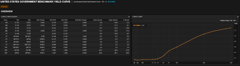
N.B.: It is important to note that the reason we can easily formulate NPV (and FV) in only two cases where $m \geq 1$ and $m < 1$ is because all maturities greater than 1 are a multiple of 1 (i.e.: they are whole numbers) (i.e.: no maturities past 1 year stop mid year, e.g.: 10 years and 6 months).
Therefore: a T-bill that matures in one month (One-month T-Bill, OMTB) has a Net Present Value:
$$ \begin{array}{ll} {NPV}_{\text{OMTB}, t} &= \begin{Bmatrix} \frac{{FV}_{\text{OMTB}, t}}{({1+{YTM}_{\text{OMTB}, t}})^{m_{\text{OMTB}}}} + \sum^{^\frac{m_{\text{OMTB}}}{f_{\text{OMTB}}}}_{\tau=1} {\frac{f_{\text{OMTB}} \text{ } C_{{\text{OMTB}}, \tau}}{ (1 + f_{\text{OMTB}} \text{ } YTM_{{\text{OMTB}},t})^{\tau} }} & \text{if } m_{\text{OMTB}} \geq 1 \\ \\ \frac{{FV}_{\text{OMTB}, t}}{{1+ \text{ } m_{\text{OMTB}} \text{ } {YTM}_{\text{OMTB}, t}}} & \text{if } m_{\text{OMTB}} < 1 \end{Bmatrix} \\ \\ &= \frac{1000 \text{ U.S.D.}}{{1+\frac{1}{12} {YTM}_{\text{OMTB}, t}}} \end{array}$$
$\text{since } m_{\text{OMTB}} = \frac{1}{12} < 1$ and ${FV}_{\text{OMTB}, t} = $ 1000 U.S.D.; all US bonds have a $FV$ of 1000 U.S.D.. Lets use the $YTM_{OMTB}$ for the 13$^\text{rd}$ of July 2020 (2020-07-13) quoted on Datastream under TRUS1MT: 0.112 U.S.D.. It is quoted in U.S.D. because it was normalised for every U.S.D.. This gives a YTM of 0.00112 (i.e.: 0.112%). Then:
$$ \begin{array}{ll} {NPV}_{\text{OMTB}, t} &= \frac{1000 \text{ U.S.D.}}{{1+\frac{1}{12} {YTM}_{\text{OMTB}, t}}} \\ & = \frac{1000 \text{ U.S.D.}}{{1+\frac{1}{12} 0.00112}} \\ & \approx 999.906675 \text{ U.S.D.} \end{array}$$
since:
1000 / (1 + (1/12) * 0.00112)
999.906675376965
(1000 - 900)/900
That - itself - is a straight-line / arithmetic daily return rate of $\frac{0.\dot{1}}{30} = 0.0\dot{0}3\dot{7} \approx 0.37 \%$ since:
((1000 - 900)/900)/30
0.0037037037037037034
(S)He theoretically gets that return every day (theoretically since it doesn't realise until the bond matures, i.e.: until the end of the Bond).
But investors are in the habit of re-investing their returns to benefit from compounding. This way we are not looking at straight-line / arithmetic interests, but geometric interest. The geometric daily interest of our investor is
since:
((1 + ((1000-900)/900)))**(1/30) - 1
0.0035181915469957303
(note that the ${\frac{1}{n}}^{th}$ exponent of a value is its $n^{th}$ root; this is a concept that is imperative to comprehend to understand the coding we go through bellow) meaning that (s)he gets approximately $900 * 0.0035 = 3.15$ USD the first day, then $(900 + 3.15) * 0.0035 \approx 3.16$ USD the next day, and so on.
Following the same logic, it is easy to calculate the risk-free rate ($r_f$) on any frequency. The compounding $r_f$ of our 1-Month T-Bill for any number of periods in a year (say, daily, i.e.: $d$) with a yield ${YTM}_{\text{OMTB}, t}$ is such that:
It is this simple because YTMs are annualised. E.g.: for a year with 252 trading days where ${YTM}_{\text{OMTB}, t} = 0.00091$ : $$r_f = \sqrt[252]{1 + 0.00091} - 1 \approx 0.0000036094755657689603 \approx 0.0004 \%$$ since:
(1.00091**(1/252))-1
3.6094755657689603e-06
This is the YTM implied daily risk-free rate ($r_f$) of our bond. A similar 'weekly' - 7 day - or 'monthly' - 30 day - rate can be made by letting $d$ be the number of weeks or months for the year in question.
Why would one use 30 days (as per our example)? Because the 1-, 2-, and 3-month rates are equivalent to the 30-, 60-, and 90-day dates respectively, reported on the Board's Commercial Paper Web page. This is as per reference (see more here and here) with that said, one ought to use the exact number of days to maturity.
Note - however - that We only looked at Zero-Coupon Bonds. If $m > 1$, then Coupons usually have to be taken into account.
We can create an R function to compute such Zero-Coupn Bond (ZCB) Yield To Maturity (YTM) Implied Risk Free Interest Rate:
ZCB_YTM_Implied_r_f = function(CMR, Maturity, D){
# This R function returns the Zero-Coupn Bond (ZCB) Yield To Maturity (YTM) Implied Risk Free Interest Rate, thus its name 'ZCB_YTM_Implied_r_f'
# CMR (vector): The Constant Maturity Rate of the Zero-Coupon Bond in question.
# Maturity (float): The number of years until the bond matures.
# This can be lower than 1, e.g.: One-Month Zero-Coupon Bonds would have a 'Maturity' value of 1/12.
# E.g.: Maturity = 1/12
# D (int): The number of time periods (e.g.: days) until the bond matures
# N.B.: The 1-, 2-, and 3-month rates are equivalent to 30-, 60-, and 90-day dates respectively, as reported on the Board's Commercial Paper Web page.
# E.g.: D = 30
# Calculate the YTM
YTM = CMR/100
# Calculate the r_f
r_f = (((YTM + 1)^Maturity)^(1/D))-1
# return a list including r_f 0th and YTM 1st.
return(r_f)}
1st: As aforementioned, the 1-, 2-, and 3-month rates are equivalent to the 30-, 60-, and 90-day dates respectively, reported on the Board's Commercial Paper Web page. This is as per reference (see more here and here). Figures are annualized using a 360-day year or bank interest. We are using Refinitiv's Datastream Constant Maturity Rate (CMR) data, more info on Constant Maturity and One-Year Constant Maturity Treasury can be found on Investopedia online and here.
2nd: From there, we workout bellow the unit return from holding a one-month Treasury bill over the period from t-1 to t by calculating its difference in daily price where: $$ Daily Price = 1000 \left[ {\left( \frac{CMR}{100} + 1 \right)}^{-\frac{1}{12}} \right] $$ Where $CRM=$ Constant Maturity Rate (i.e.: TRUS1MT, TRUS3MT, or TRUS10T). The price of the theoretical risk-free asset in our case is: $$ P_{r_{f_{SPX}},t} = 1000 \left[ \left( \frac{TRUS1MT_t}{100} + 1 \right)^{-\frac{1}{12}} \right] $$ and we define
where $t \in \mathbb{Z}$ and $ 1 \le t \ge T_{US\_1MO\_r\_f}$. We define the (time) vector
$ \mathbf{US\_1MO\_r\_f} = $ $ \left[ \begin{matrix} r_{{f_{SPX}},1} \\ r_{{f_{SPX}},2} \\ \vdots\\ r_{{f_{SPX}},T_{US\_1MO\_r\_f}} \end{matrix} \right] $
$\mathbf{US\_1MO\_r\_f}$ is thus as defined in the cell bellow.
US_1MO_r_f = ((((((TRUS1MT_raw/100)+1)^(-1/12))*1000) -
((((lag(TRUS1MT_raw)/100)+1)^(-1/12))*1000)) /
((((lag(TRUS1MT_raw)/100)+1)^(-(1/12)))*1000))
US_1MO_r_f_zoo = zoo(US_1MO_r_f) # Calculations and manipulations of ' US_1MO_r_f ' nessesitate it to be a 'zoo' R variable.
colnames(US_1MO_r_f_zoo) = "US_1MO_r_f"
If you are havving issues with vector lengths, try running the cell above replacing ' lag ' with ' stats::lag '
Let's have a look at what our latest data input looks like:
Spec_Table(US_1MO_r_f_zoo)
We will construct a referential Data-Frame, ' df ':
df = na.omit(merge(x = df, y = US_1MO_r_f_zoo, all = TRUE))
This is what a row of our Data-Frame looks like at the moment:
print(df[c("2006-04-05"),])
$R_t$ (and its lagged value, $R_{t-1}$)
The SPX's index excess returns at time t are computed as per CPV, Pesaran and Timmermann (1995) and Chevapatrakul (2013) for each index such that:
$$\begin{equation} R_{SPX, t} = \frac{P_{SPX, t} - P_{SPX, t-1}}{P_{SPX, t-1}} - {r_{f_{SPX, t}}} \end{equation}$$Note here that:
1st: Due to the differencing nessesary to calculate 'R', the first value is empty. The following command displays this well:
as.matrix(((SPX_df-lag.xts(data.matrix(SPX_df)))/SPX_df)-US_1MO_r_f_r_f)
2nd: In order for the correct SPX_R values to be associated with the correct dates, the element SPX_R has to be changed into a 'zoo' element. This will allow future models to have data points with correct date labels. A vector element is left however, for libraries and functions that do not support them.
We define the (time) vector
$\mathbf{SPX_R} = \left[ \begin{matrix} R_{SPX, 1} \\ R_{SPX, 2} \\ \vdots\\ R_{SPX, T_{SPX\_R}} \end{matrix} \right] $
SPX_R = as.matrix(((zoo(SPX_raw)-lag.xts(zoo(SPX_raw))) / lag.xts(zoo(SPX_raw))) - zoo(US_1MO_r_f))
# the use of ' zoo() ' is a trick to make sure that only compatible data is manipulated.
# This far in our article we wouldn't need it, but it is better to generalise for other senarios.
colnames(SPX_R) = "SPX_R"
We will construct a referential Data-Frame, ' df ':
df = na.omit(merge(x = df, y = zoo(SPX_R, as.Date(row.names(SPX_R))), all = TRUE))
Let's have a look at what our latest data input looks like:
Spec_Table(SPX_R)
Note that due to the use of a lagged variable ($t-1$), the 1st value of $\mathbf{SPX\_R}$ is empty
As per Barndorff-Nielsen and Shephard (2002), Realised Volatility (Andersen, Bollerslev, Diebold, and Ebens (2001)) has been shown to be an accurate, useful and model-free representation of volatility in the literature. I therefore use it as a benchmark against which to assess volatility forecasts.
The SPX close-prices ($P_{SPX}$) as well as their 5 minute subsampling Realised-Variances ($RVAR_{SPX}$ and $RV_{SPX}$) are Refinitiv data-sets compiled and collected from the Realized Library of the Oxford-Man Institute. Realised Volatilities at time t are computed as
$ \begin{equation} {RV}_{SPX, t} = \sqrt{{RVAR}_{SPX, t}} \end{equation} $
where
$ \mathbf{SPX\_RV} = \left[ \begin{matrix} {RV}_{SPX, 1}\\ {RV}_{SPX, 2}\\ \vdots\\ {RV}_{SPX, T_{SPX\_RV}} \end{matrix} \right] = \left[ \begin{matrix}\sqrt{{RVAR}_{SPX, 1}}\\ \sqrt{{RVAR}_{SPX, 2}}\\ \vdots\\ \sqrt{{RVAR}_{SPX, T_{SPX\_RV}}} \end{matrix} \right] $
and where $t \in \mathbb{Z}$ and $ 1 \le t \ge T_{SPX\_RV}$.
Nota Bene (N.B.): $\sqrt{x} = x^{0.5}$ $\forall x \in \mathbb{R}$ and that $\mathbb{Z} \subset \mathbb{R}$
current_directory = toString(getwd())
# First we setup dates:
SPX_Dates_df = read_excel(
toString(
paste(
current_directory,
"/Data/1-Month_Treasury_Rate/1-Month_Treasury_Constant_Maturity_Rate_FRED_id_DGS1MO_2004.01.01_to_2019.03.13.xlsx",
sep = "")),
sheet = "Without_FRED_or_O-M_Holidays",
range = "A2:A3794",
col_names = "SPX_Dates")
SPX_Dates = as.Date(SPX_Dates_df$SPX_Dates,"%Y-%m-%d", tz="Europe/London")
# Then setup the Variance:
SPX_RVar_df = read_excel(
toString(
paste(
current_directory,
"Data/Realised Volatility/5min_realised_volatility_from_Oxford-Man.xlsx",
sep = "")),
sheet = "SPX2004-2019.03.1WithoutFREDHol",
range = "I2:I3794",
col_names = "SPX_RVar")
# Note that the Ox-Man institute provides real VARIANCE as per
# https://realized.oxford-man.ox.ac.uk/documentation/estimators
SPX_RV_df = (SPX_RVar_df^0.5)
SPX_RV = as.matrix(SPX_RV_df)
colnames(SPX_RV) = c('SPX_RV')
SPX_RV_zoo = zoo(SPX_RV, as.Date(SPX_Dates))
Let's have a look at what our latest data input looks like:
Spec_Table(SPX_RV)
We will construct a referential Data-Frame, ' df ':
df = na.omit(merge(x = df, y = SPX_RV_zoo, all = TRUE))
This is what a row of our Data-Frame looks like at the moment:
print(df[c("2006-04-05"),])
S.PCOMP TRUS1MT TRUS3MT TRUS10T US_1MO_r_f SPX_R SPX_RV
2006-04-05 1311.56 4.54 4.656 4.843 1.195636e-05 0.004299148 0.005001079
Alphabet Inc.'s Google Trends tool provides the number of times a specified term was searched on their website - for specified world regions and time-periods - normalised from 0 to 100, forming the SVI. In this article, SVI was gathered as outlined in CPV's Appendix A, normalising all results such that the day the term was searched the most in the period of choice is valued as 100 and the least as 0.
The worldwide searched term used as an SVI keyword here is "s&p 500” - rendering $SVI_{SPX}$. This is in line with Vlastakis and Markellos (2012) and their study on the best terms to use in such investigations. They used several variations of the index term in addition to ones proposed by Wordtracker. (Wordtracker offers Search Engine word search reports that include related search terms.) This study suggested picking the one with greatest search volume in the sample period. This is - naturally - in addition to picking no terms that may easily be misconstrued and have other meanings (e.g.: the listed company name 'Apple' which may also refer to the apple fruit).
We denote $$ \Delta SVI_{SPX, t} = SVI_{SPX, t} - SVI_{SPX, t-1} $$ where $t \in \mathbb{Z}$ denotes only trading days.
For completeness, I repeated my work relaxing $SVI_{SPX, t-1}$'s time set to any day, not only trading days, while keeping $SVI_{SPX, t}$'s strictly to trading days to allow for situations where, e.g., $t$ would denote a Monday and $t-1$ a Sunday. Equally, I repeated my work on all $SVI_{SPX}$ moving averages from 2 days to one week.
All $SVI_{SPX}$ data represented Worldwide results.
We thus define
$ \mathbf{SPX\_dSVI} =$ $ \left[ \begin{matrix} {\Delta SVI}_{SPX, 1}\\ {\Delta SVI}_{SPX, 1}\\ \vdots\\ {\Delta SVI}_{SPX, T_{SPX\_dSVI}} \end{matrix} \right] $
where $t \in \mathbb{Z}$ and $ 1 \le t \ge T_{SPX\_dSVI}$ as per the bellow:
- 1st: Gather $SVI_t$ data
# The SVI Excel file tends to have empty values at its end.
# The 'slice' function bellow will remove them.
SPX_SVI_df = slice(
read_excel(
"C:/Users/U6082174.TEN/OneDrive - Refinitiv/UoE/Disertation/Data/SVI/SVI_from_2004.01.01_to_2019.03.13_normalised_by_2018.02.06_Only_Trading_Days.xlsx",
sheet = "SVI_Without_O-M_Holidays",
range = "A1:B3802",
col_names = c("Dates", "SPX_SVI")),
1:length(SPX_Dates))
SPX_SVI = as.matrix(SPX_SVI_df$SPX_SVI) # Convert the data frame 'SPX_SVI_df' into a matrix
SPX_SVI_zoo = zoo(SPX_SVI, as.Date(SPX_SVI_df$Dates,"%Y-%m-%d", tz="Europe/London"))
colnames(SPX_SVI_zoo) = "SPX_SVI"
let's have a look at its characteristics:
Spec_Table(SPX_SVI_zoo)
let's add this to our data-frame:
df = na.omit(merge(x = df, y = SPX_SVI_zoo, all = TRUE))
- 2nd: Now make $dSVI_t$ values
# Construct Google's Search Vecrot Index (SVI).
SPX_dSVI = zoo(SPX_SVI_zoo - lag.xts(data.matrix(SPX_SVI_zoo)))
colnames(SPX_dSVI) = "SPX_dSVI"
Spec_Table(SPX_dSVI)
df = na.omit(merge(x = df, y = SPX_dSVI, all = TRUE))
SPX_R = zoo(as_tibble(df, rownames = NA) %>% select(SPX_R))
Spec_Table(SPX_R)
Let's graph our SVI data:
par(bg = "grey30", col.axis = "white", col.lab = "white", col.main = "white", col.sub = "white")
plot(SPX_SVI_zoo, xlab = 'Date', ylab = "SPX's SVI", col = "blue", type = 'l',
main = "Google's Search Vector Index for the searched term 's&p 500'")
/googles_search_vector_index.png.transform/resize-768/q82/image.png)
One can identify several key dates at peaks in the figure above. Interestingly, it shows three peaks that did not show in CVP (06/02/2018 and 09/02/2018), the days following the (more than) doubling of the fear-gauge Chicago Board Options Exchange Volatility Index (Economist (8th of Febuary 2018)); and 26/12/2018, when tensions between the U.S. Federal Bank Chair and the Government's President were revealed as impactful.
It is important to note several caveats with SVIs. First, SVI data has randomised elements so as to stop any individual form identifying any one particular person or group's internet searches.
Second, we must not forget that while Google's implementation of caffeine (Dave Davis (2017)) on 08/06/2010 may have distorted SVI data little enough for CPV's work in 2017/2018, it may also have accumulated by 13/03/2019, rendering this dataset less consistent from year to year. To circumvent such issues, one might consider using other metrics (such as Reuters News) or splitting the sample into two (pre and post caffeine implementation).
par(bg = "grey30", col.axis = "white", col.lab = "white", col.main = "white", col.sub = "white")
epdfPlot(as.numeric(SPX_R), main = "", xlab = "", epdf.col = "orange2")
pdfPlot(param.list = list(mean=0, sd = sd(na.omit(SPX_R))), add = TRUE, pdf.col = "blue")
pdfPlot(add = TRUE, pdf.col = "green4")
legend("topright", legend = c("EPDF plot of Excess SPX Returns", "N[0,Var(Excess SPX Returns)]", "N(0,1)"),
col = c("orange2", "blue", "green4"), text.col = c("white"), lwd = 2 * par("cex"))
title("Probability Distribution Function Plots")
/probability_distribution_function_plots.png.transform/resize-768/q82/image.png)
This PDF graph allows us to discern SPX_R's leptokurtoticity as anticipated by SFFR (i). One may also note the skewness that allows for the application of CDMTT's work.
rbind(Statistics_Table("US_1MO_r_f_zoo", na.omit(US_1MO_r_f_zoo)),
Statistics_Table("SPX_R", na.omit(SPX_R)),
Statistics_Table("SPX_RV", SPX_RV_zoo),
Statistics_Table("SPX_SVI", SPX_SVI), # Note that SVIFTSE_zoo's Mean is the same as 'mean(SPX_dSVI_zoo)'; after much study on the matter, it seems as though this mean and other statistics are correct, which only highlights how different seperate SVI draws can be.
Statistics_Table("SPX_dSVI", na.omit(SPX_dSVI)))
This statistics table allows us to discern SPX_R's leptokurtoticity again - as anticipated by SFFR (i). One may also note the skewness that allows for the application of CDMTT's work - yet again.
dSVI's ACFs also provide us with evidence that they are stationary. The concept of stationarity and its necessity is explained in Part 2. For more on the necessity of stationary variables in research such as this one, see Verbeek (2008) Chapters 8 to 10.
Bellow, we perform an Augmented Dickey-Fuller Test:
print("Augmented Dickey-Fuller Test of SPX's SVI")
adf.test(matrix(SPX_SVI), nlag = NULL, output = TRUE) # Our ADF test here should show that we reject the Null Hypothesis (low p-value) in preference for the alternative of stationarity. One can see that dSVIFTSE_zoo is stationary by ploting it with:
[1] "Augmented Dickey-Fuller Test of SPX's SVI"
Augmented Dickey-Fuller Test
alternative: stationary
Type 1: no drift no trend
lag ADF p.value
[1,] 0 -8.13 0.0100
[2,] 1 -5.76 0.0100
[3,] 2 -4.55 0.0100
[4,] 3 -3.92 0.0100
[5,] 4 -3.69 0.0100
[6,] 5 -3.33 0.0100
[7,] 6 -3.05 0.0100
[8,] 7 -2.69 0.0100
[9,] 8 -2.41 0.0172
Type 2: with drift no trend
lag ADF p.value
[1,] 0 -16.20 0.01
[2,] 1 -11.69 0.01
[3,] 2 -9.32 0.01
[4,] 3 -8.16 0.01
[5,] 4 -7.75 0.01
[6,] 5 -7.13 0.01
[7,] 6 -6.62 0.01
[8,] 7 -5.97 0.01
[9,] 8 -5.39 0.01
Type 3: with drift and trend
lag ADF p.value
[1,] 0 -19.65 0.01
[2,] 1 -14.38 0.01
[3,] 2 -11.64 0.01
[4,] 3 -10.26 0.01
[5,] 4 -9.81 0.01
[6,] 5 -9.05 0.01
[7,] 6 -8.46 0.01
[8,] 7 -7.67 0.01
[9,] 8 -7.02 0.01
----
Note: in fact, p.value = 0.01 means p.value <= 0.01
SVI's Augmented Dickey-Fuller (ADF) (Dickey and Fuller (1979)) tests indicate a rejection of the null in preference for the alternative of stationarity at the 99% Confidence Level (CL).
Bellow we perform a KPSS test:
print("KPSS Test of SPX_SVI_zoo")
kpss.test(matrix(SPX_SVI_zoo))
[1] "KPSS Test of SPX_SVI_zoo"
KPSS Unit Root Test
alternative: nonstationary
Type 1: no drift no trend
lag stat p.value
14 27.2 0.01
-----
Type 2: with drift no trend
lag stat p.value
14 9.41 0.01
-----
Type 1: with drift and trend
lag stat p.value
14 3.26 0.01
-----------
Note: p.value = 0.01 means p.value <= 0.01
: p.value = 0.10 means p.value >= 0.10
The KPSS (Kwiatkowski–Phillips–Schmidt–Shin) tests are used for testing a null hypothesis that an observable time series is stationary around a deterministic trend against the alternative of a unit root. It similarly indicates that our SVI dataset is stationary.
As per the outlined methods, we will use the 1st difference in SVI in our models. If SVI is stationary, then dSVI is too, making it compatible with our work.
Saving our data this far to help with de-bugging if needed: (It start with p4 as I ran debugging sessions 4 times by this point; I would advise anyone doing such a study necessitating a large amount of data computation to regularly save data progression in files using a logical naming procedure)
save.image(file = "IDaSRP_work_space_p4.00.01.RData")
# To restore your workspace, type this:
# load("IDaSRP_work_space_p4.00.01.RData")
Next, we will look into the Econometric Modelling of Non-Linear Variances in Part 2. In this section - as aforementioned - there is no coding. Instead we go – step by step and including working outs – through ARMA models, their parameter estimation process (via log-likelihood), the concepts of stationarity, Taylor’s expansion, the calculus’ chain rule, first order conditions, and GARCH models (including the GACH, GJRGARCH and EGARCH models). Finally, we outline the way in which we construct error values from which to evaluate the performance of our models.
References
You can find more detail regarding the DSWS API and related technologies for this article from the following resources:
- DSWS page on the Refinitiv Developer Community web site.
- DSWS API Quick Start Guide page.
- DSWS Tutorial page.
- DSWS API Python Reference Guide.
- DSWS in R
For any questions related to this article or the DSWS API, please use the Developers Community Q&A Forum.
Related Articles