
Overview
Technical Analysis for intraday trading is one of the basic approaches to help you choose the planning of ventures. Basically, users can use the intraday or end-of-day pricing data to generate charts such as the CandleStick. They can then review the stock price' trend and make decisions using their own method or algorithm. Typically, Refinitiv Workspace and Eikon Desktop users also provide access to this information, and it also provides a user interface to display multiple types of Charts.
However, there is a specific requirement from a customer who did not use Eikon or Refinitiv Workspace. They need to build their own stand-alone application or generate the charts on their application using data from Refintiv. The user is looking for the source of data or service to provide the intraday data for them in the REST API format. So they can integrate the service with their app.
To support the requirement client can use REST API provided by Refinitiv Data Platform (RDP) that basically provides simple web-based API access to a broad range of content provided by Refinitiv. It can retrieve data such as News, ESG, Symbology, Streaming Price, and Historical Pricing. Users can get the intraday from the Historical Pricing service and then pass the data to any libraries that provided functionality to generate Charts. To help API users access RDP content easier, Refinitiv also provides the Refinitiv Data Platform (RDP) Libraries that provide a set of uniform interfaces providing the developer access to the Refinitiv Data Platform. We are currently providing an RDP Library for Python and .NET users. A general user and data scientists can leverage the library's functionality to retrieve data from the service, which basically provides the original response message from the RDP service in JSON tabular format. The RDP Library for Python will then convert the JSON tabular format to the pandas dataframe so that the user does not need to handle a JSON message and convert it manually. The user can use the dataframe with libraries such as the mathplotlib and mplfinance library to display the Charts.
In this example, I will show you how to use RDP Library for Python, request the intraday data from the Historical Pricing service, and then generate basic charts such as the Candle Stick and OHLC charts. Basically, the Japanese candlestick chart is commonly used to illustrate movements in a financial instrument's price over time. It's popular in finance, and some technical analysis strategies use them to make trading decisions, depending on the candles' shape, color, and position.
Prerequisites
Follow instructions from Quick Start Guide to install RDP Library for python.
> pip install refinitiv.dataplatform
You must have RDP Account with permission to request data using Historical Pricing API. You can also login to the APIDocs page. Then you can search for the Historical Pricing and looking at section Reference for the document.
Ensure that you have the following additional python libraries.
configparser, matplotlib, mplfinance, seaborn
Getting Started using RDP API for python
I will create a configuration file to keep the RDP user info and read it using ConfigParser. This module provides a class that implements a basic configuration language that provides a structure similar to what’s found in Microsoft Windows INI files. We will start creating a configuration file name rdp_cofig.cfg. It will contain the rdpuser section, which use to keep app_key, username, and password.
Below is a sample configuration file you must create.
[rdpuser]
app_key = <Appkey/ClientId>
username = <RDP User>
password = <RDP Password>
Open the Platform Session
Next step, we will import refinitiv.dataplatform library and pass RDP user to function open_platform_session to open a session to the RDP server. RDP library will handle the authorization and manage the session for you.
import refinitiv.dataplatform as rdp
import configparser as cp
global session
global ricName
session=None
cfg = cp.ConfigParser()
#change cfgpath to your own path on your OS.
cfgpath= './rdp_config.cfg'
if not cfg.read(cfgpath) :
print(f'Unable to read the configuration file')
else:
print(f"RDP Version {rdp.__version__}")
# Open RDP Platform Session
print("Open Platform Session")
session = rdp.open_platform_session(cfg['rdpuser']['app_key'],rdp.GrantPassword(username = cfg['rdpuser']['username'],password = cfg['rdpuser']['password']))
print(f"RDP Sesssion State is now {session.get_open_state()}")
RDP Version 1.0.0a7
Open Platform Session
RDP Sesssion State is now State.Open
Retrieve Time Series data from RDP
After the session state is Open, we will use the below get_historical_price_summaries interface to retrieve time series pricing Interday summaries data(i.e., bar data).
get_historical_price_summaries(universe, interval=None, start=None, end=None, adjustments=None, sessions=[], count=1, fields=[], on_response=None, closure=None)
Actually, the implementation of this function will send HTTP GET requests to the following RDP endpoint.
https://api.refinitiv.com/data/historical-pricing/v1/views/interday-summaries/
And the following details are possible values for interval and adjustment arguments.
Supported intervals: Intervals.DAILY, Intervals.WEEKLY, Intervals.MONTHLY, Intervals.QUARTERLY, Intervals.YEARLY.
Supported value for adjustments: 'unadjusted', 'exchangeCorrection', 'manualCorrection', 'CCH', 'CRE', 'RPO', 'RTS', 'qualifiers'
You can pass an array of these values to the function like the below sample codes.
adjustments=['unadjusted']
adjustments=['unadjusted','CCH','CRE','RPO','RTS']
Please find below details regarding the adjustments behavior; it's the details from a reference section on the APIDocs page. Note that it can be changed in future releases. I would suggest you leave it to the default value.
The adjustments are a query parameter that tells the system whether to apply or not apply CORAX (Corporate Actions) events or exchange/manual corrections or price and volume adjustment according to trade/quote qualifier summarization actions to historical time series data.
Normally, the back-end should strictly serve what clients need. However, if the back-end cannot support them, the back-end can still return the form that the back-end supports with the proper adjustments in the response and status block (if applicable) instead of an error message.
Limitations: Adjustment behaviors listed in the limitation section may be changed or improved in the future.
If any combination of correction types is specified (i.e., exchangeCorrection or manualCorrection), all correction types will be applied to data in applicable event types.
If any CORAX combination is specified (i.e., CCH, CRE, RPO, and RTS), all CORAX will be applied to data in applicable event types.
Adjustments values for Interday-summaries and Intraday-summaries API
If unspecified, each back-end service will be controlled with the proper adjustments in the response so that the clients know which adjustment types are applied by default. In this case, the returned data will be applied with exchange and manual corrections and applied with CORAX adjustments.
If specified, the clients want to get some specific adjustment types applied or even unadjusted.
The supported values of adjustments:
- exchangeCorrection - Apply exchange correction adjustment to historical pricing
- manualCorrection - Apply manual correction adjustment to historical pricing, i.e., annotations made by content analysts
- CCH - Apply Capital Change adjustment to historical Pricing due to Corporate Actions, e.g., stock split
- CRE - Apply Currency Redenomination adjustment when there is a redenomination of the currency
- RTS - Apply Reuters TimeSeries adjustment to adjust both historical price and volume
- RPO - Apply Reuters Price Only adjustment to adjust historical price only, not volume
- unadjusted - Not apply both exchange/manual correct and CORAX
Notes:
Summaries data will always have exchangeCorrection and manualCorrection applied. If the request is explicitly asked for uncorrected data, a status block will be returned along with the corrected data saying, "Uncorrected summaries are currently not supported".
The unadjusted will be ignored when other values are specified.
Below is a sample code to retrieve Daily historical pricing for the RIC defined in the ricName variable, and I will set the start date from 2013 to nowaday. You need to set the interval to rdp.Intervals.DAILY to get intraday data. We will display the column's name with the heads and tails of the dataframe to review the data.
import pandas as pd
import datetime
from IPython.display import clear_output
ricName='MSFT.O'
StartDate = '2010.01.01'
EndDate = str(datetime.date.today())
if session != None :
data = rdp.get_historical_price_summaries(
universe = ricName,
interval = rdp.Intervals.DAILY, # Supported intervals: DAILY, WEEKLY, MONTHLY, QUARTERLY, YEARLY.
start=StartDate, end= EndDate)
if data is not None:
#Show information of the dataframe to see column name , null and null-null field and the data type of the column
data.info()
display(data.head)
display(data.tail)
else:
print("Error while process the data")
Sample Output
<class 'pandas.core.frame.DataFrame'>
DatetimeIndex: 2795 entries, 2009-12-31 to 2021-02-08
Data columns (total 15 columns):
# Column Non-Null Count Dtype
--- ------ -------------- -----
0 TRDPRC_1 2795 non-null float64
1 HIGH_1 2795 non-null float64
2 LOW_1 2795 non-null float64
3 ACVOL_UNS 2795 non-null Int64
4 OPEN_PRC 2795 non-null float64
5 BID 2795 non-null float64
6 ASK 2795 non-null float64
7 TRNOVR_UNS 1621 non-null float64
8 VWAP 2795 non-null float64
9 BLKCOUNT 2795 non-null Int64
10 BLKVOLUM 2795 non-null Int64
11 NUM_MOVES 2343 non-null Int64
12 TRD_STATUS 1399 non-null Int64
13 SALTIM 1387 non-null Int64
14 NAVALUE 0 non-null object
dtypes: Int64(6), float64(8), object(1)
memory usage: 365.8+ KB
<bound method NDFrame.head of TRDPRC_1 HIGH_1 LOW_1 ACVOL_UNS OPEN_PRC BID ASK \
2009-12-31 30.480 30.9900 30.48 31929611 30.9799 30.48 30.50
2010-01-04 30.950 31.1000 30.59 38414185 30.6200 30.94 30.95
2010-01-05 30.960 31.1000 30.64 49758862 30.8500 30.94 30.95
2010-01-06 30.770 31.0800 30.52 58182332 30.8800 30.76 30.77
2010-01-07 30.452 30.7000 30.19 50564285 30.6300 30.47 30.48
... ... ... ... ... ... ... ...
2021-02-02 239.510 242.3100 238.69 25916337 241.3000 239.47 239.48
2021-02-03 243.000 245.0900 239.26 27158104 239.5700 242.94 243.00
2021-02-04 242.010 243.2399 240.37 25296100 242.6600 241.91 242.12
2021-02-05 242.200 243.2800 240.42 18054752 242.2300 242.20 242.22
2021-02-08 242.470 243.6800 240.81 22211929 243.1500 242.47 242.52
TRNOVR_UNS VWAP BLKCOUNT BLKVOLUM NUM_MOVES TRD_STATUS \
2009-12-31 NaN 30.7090 88 6866420 <NA> <NA>
2010-01-04 NaN 30.9712 103 8249383 <NA> <NA>
2010-01-05 NaN 30.9207 123 8968509 <NA> <NA>
2010-01-06 NaN 30.7796 134 8942497 <NA> <NA>
2010-01-07 NaN 30.3920 134 7848431 <NA> <NA>
... ... ... ... ... ... ...
2021-02-02 6.226880e+09 240.2895 51 4843599 299116 1
2021-02-03 6.593201e+09 242.7943 46 4958652 289329 1
2021-02-04 6.107954e+09 241.4004 48 5310115 269884 1
2021-02-05 4.364354e+09 241.6822 36 3600568 218266 1
2021-02-08 5.378323e+09 242.0355 36 8408789 219524 1
SALTIM NAVALUE
2009-12-31 <NA> None
2010-01-04 <NA> None
2010-01-05 <NA> None
2010-01-06 <NA> None
2010-01-07 <NA> None
... ... ...
2021-02-02 75600 None
2021-02-03 75600 None
2021-02-04 75600 None
2021-02-05 75600 None
2021-02-08 75600 None
[2795 rows x 15 columns]>
<bound method NDFrame.tail of TRDPRC_1 HIGH_1 LOW_1 ACVOL_UNS OPEN_PRC BID ASK \
2009-12-31 30.480 30.9900 30.48 31929611 30.9799 30.48 30.50
2010-01-04 30.950 31.1000 30.59 38414185 30.6200 30.94 30.95
2010-01-05 30.960 31.1000 30.64 49758862 30.8500 30.94 30.95
2010-01-06 30.770 31.0800 30.52 58182332 30.8800 30.76 30.77
2010-01-07 30.452 30.7000 30.19 50564285 30.6300 30.47 30.48
... ... ... ... ... ... ... ...
2021-02-02 239.510 242.3100 238.69 25916337 241.3000 239.47 239.48
2021-02-03 243.000 245.0900 239.26 27158104 239.5700 242.94 243.00
2021-02-04 242.010 243.2399 240.37 25296100 242.6600 241.91 242.12
2021-02-05 242.200 243.2800 240.42 18054752 242.2300 242.20 242.22
2021-02-08 242.470 243.6800 240.81 22211929 243.1500 242.47 242.52
TRNOVR_UNS VWAP BLKCOUNT BLKVOLUM NUM_MOVES TRD_STATUS \
2009-12-31 NaN 30.7090 88 6866420 <NA> <NA>
2010-01-04 NaN 30.9712 103 8249383 <NA> <NA>
2010-01-05 NaN 30.9207 123 8968509 <NA> <NA>
2010-01-06 NaN 30.7796 134 8942497 <NA> <NA>
2010-01-07 NaN 30.3920 134 7848431 <NA> <NA>
... ... ... ... ... ... ...
2021-02-02 6.226880e+09 240.2895 51 4843599 299116 1
2021-02-03 6.593201e+09 242.7943 46 4958652 289329 1
2021-02-04 6.107954e+09 241.4004 48 5310115 269884 1
2021-02-05 4.364354e+09 241.6822 36 3600568 218266 1
2021-02-08 5.378323e+09 242.0355 36 8408789 219524 1
SALTIM NAVALUE
2009-12-31 <NA> None
2010-01-04 <NA> None
2010-01-05 <NA> None
2010-01-06 <NA> None
2010-01-07 <NA> None
... ... ...
2021-02-02 75600 None
2021-02-03 75600 None
2021-02-04 75600 None
2021-02-05 75600 None
2021-02-08 75600 None
[2795 rows x 15 columns]>
Preparing data for plotting chart
Next steps, we will create a new dataframe object from the data returned by the interday-summaries endpoint. We need to map the columns from the original dataframe to Open, High, Low, Close(OHLC) data. So we will define column names to map the OHLC data from the following variables.
openColumns =>Open
highColumns => High
lowColumns => Low
closeColumns => Close
volumeColums => Volume
openColumns="OPEN_PRC"
highColumns="HIGH_1"
lowColumns="LOW_1"
closeColumns="TRDPRC_1"
volumeColumns="ACVOL_UNS"
ohlc_dataframe= data[[openColumns,highColumns,lowColumns,closeColumns,volumeColumns]]
ohlc_dataframe.index.name = 'Date'
display(ohlc_dataframe)
#rename the column name
ohlc_dataframe.info()
ohlc_dataframe=ohlc_dataframe.rename(columns={openColumns:"Open",highColumns:"High",lowColumns:"Low",closeColumns:"Close",volumeColumns:"Volume"})
print(ohlc_dataframe.columns)
display(ohlc_dataframe)
Sample Output
OPEN_PRC HIGH_1 LOW_1 TRDPRC_1 ACVOL_UNS
Date
2009-12-31 30.9799 30.9900 30.48 30.480 31929611
2010-01-04 30.6200 31.1000 30.59 30.950 38414185
2010-01-05 30.8500 31.1000 30.64 30.960 49758862
2010-01-06 30.8800 31.0800 30.52 30.770 58182332
2010-01-07 30.6300 30.7000 30.19 30.452 50564285
... ... ... ... ... ...
2021-02-02 241.3000 242.3100 238.69 239.510 25916337
2021-02-03 239.5700 245.0900 239.26 243.000 27158104
2021-02-04 242.6600 243.2399 240.37 242.010 25296100
2021-02-05 242.2300 243.2800 240.42 242.200 18054752
2021-02-08 243.1500 243.6800 240.81 242.470 22211929
2795 rows × 5 columns
<class 'pandas.core.frame.DataFrame'>
DatetimeIndex: 2795 entries, 2009-12-31 to 2021-02-08
Data columns (total 5 columns):
# Column Non-Null Count Dtype
--- ------ -------------- -----
0 OPEN_PRC 2795 non-null float64
1 HIGH_1 2795 non-null float64
2 LOW_1 2795 non-null float64
3 TRDPRC_1 2795 non-null float64
4 ACVOL_UNS 2795 non-null Int64
dtypes: Int64(1), float64(4)
memory usage: 133.7 KB
Index(['Open', 'High', 'Low', 'Close', 'Volume'], dtype='object')
Open High Low Close Volume
Date
2009-12-31 30.9799 30.9900 30.48 30.480 31929611
2010-01-04 30.6200 31.1000 30.59 30.950 38414185
2010-01-05 30.8500 31.1000 30.64 30.960 49758862
2010-01-06 30.8800 31.0800 30.52 30.770 58182332
2010-01-07 30.6300 30.7000 30.19 30.452 50564285
... ... ... ... ... ...
2021-02-02 241.3000 242.3100 238.69 239.510 25916337
2021-02-03 239.5700 245.0900 239.26 243.000 27158104
2021-02-04 242.6600 243.2399 240.37 242.010 25296100
2021-02-05 242.2300 243.2800 240.42 242.200 18054752
2021-02-08 243.1500 243.6800 240.81 242.470 22211929
2795 rows × 5 columns
Visualizing Stock Data
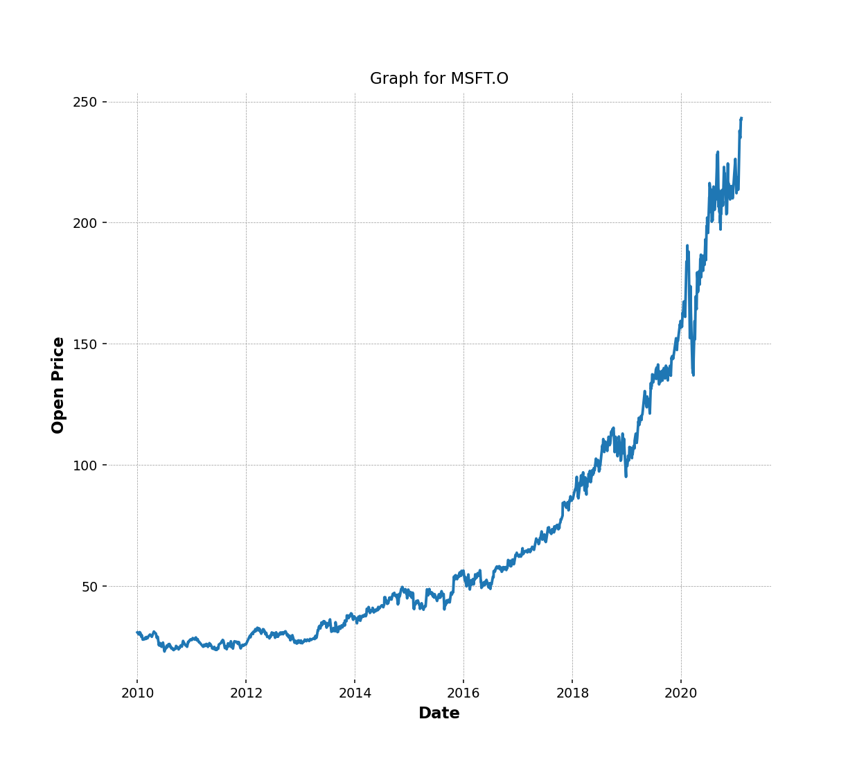
Plot a simple Daily Closing Price line graph
We can create a simple line graph to compare open and close price using the following codes. You can change the size of the figure.figsize to adjust chart size.
import matplotlib.pyplot as plt
%matplotlib notebook
fig = plt.figure(figsize=(9,8),dpi=100)
ax = plt.subplot2grid((3,3), (0, 0), rowspan=3, colspan=3)
titlename='Graph for '+ricName
ax.set_title(titlename)
ax.set_xlabel('Date')
ax.set_ylabel('Open Price')
ax.grid(True)
ax.plot(ohlc_dataframe.index, ohlc_dataframe.Open)
plt.show()
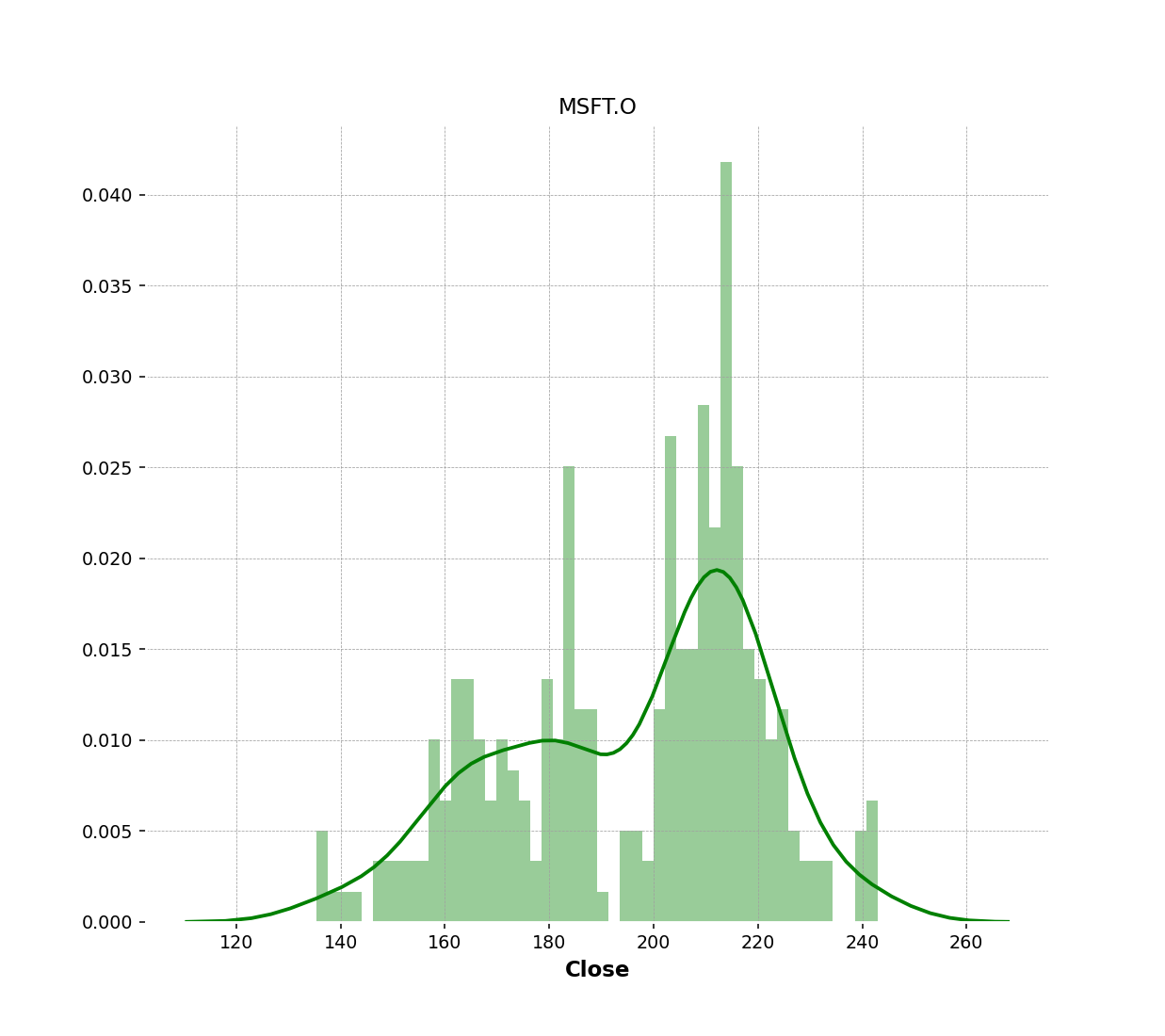
Generate a Histogram of the Daily Closing Price
We can review daily closing prices over time to see the spread or volatility and the type of distribution using the histogram. We can use the distplot method from the seaborn library to plot the graph.
import seaborn as sns
import matplotlib.pyplot as plt
plt.figure(figsize=(9,8),dpi=100)
dfPlot=ohlc_dataframe[['Close','Volume']].loc['2020-01-01':datetime.date.today(),:]
graph=sns.distplot(dfPlot.Close.dropna(), bins=50, color='green')
graph.set_title(ricName)
plt.show()
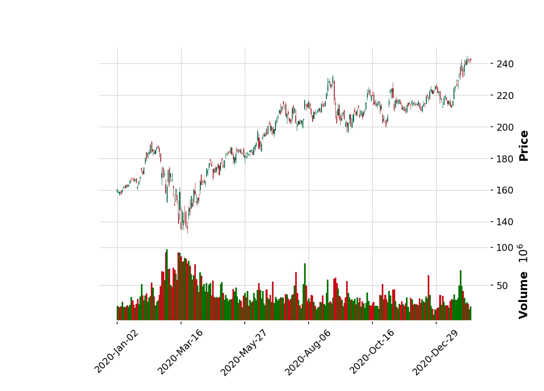
Using the mplfiance library to generate CandleStick and OHLC chart
Next step, we will generate a CandleStick and OHLC chart using the new version mplfinance library. We need to pass a dataframe that contains Open, High, Low, and Close data to the mplfinance.plot function and specify the name of the chart you want to plot.
import mplfinance as mpf
import datetime
%matplotlib notebook
ohlc_dataframe.info()
#Volume use Int64 it will returns fails when mplfinance.plot check the support type of the data.So we need to convert it to Int64 and remove na from the data frame.
#If you don't care about Volume you can drop it from the dataframe.
dfPlot=ohlc_dataframe.dropna().astype({col: 'int64' for col in ohlc_dataframe.select_dtypes('Int64').columns}).loc['2020-01-01':str(datetime.date.today())]
display(dfPlot)
dfPlot.info()
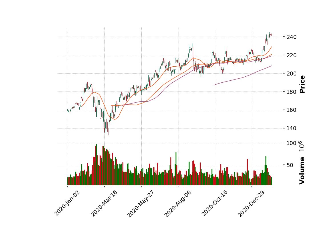
mpf.plot(dfPlot.loc[:str(datetime.date.today()),:],type='candle',style='charles',volume=True)
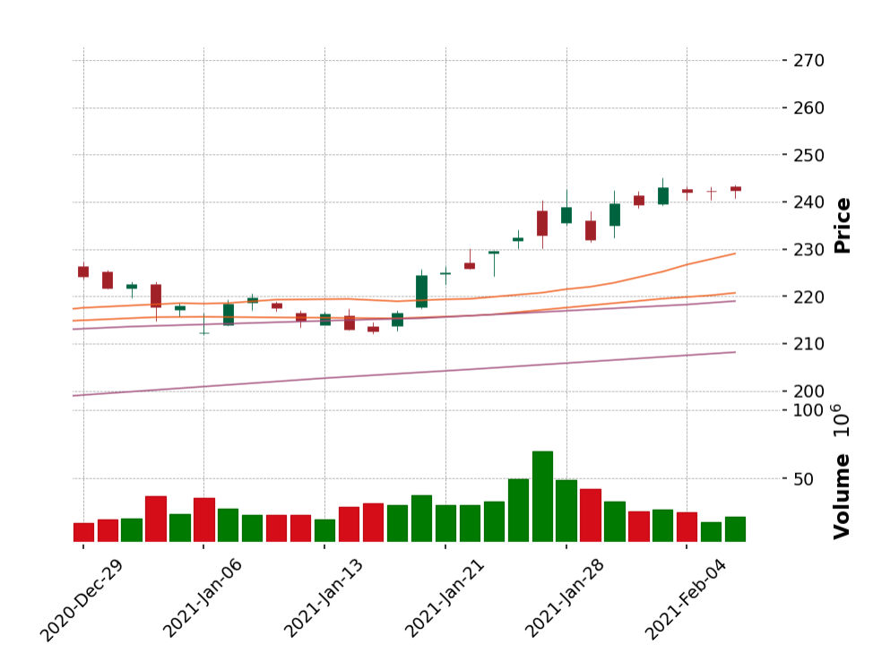
Display shorter period.
tempPlot= ohlc_dataframe.dropna().astype({col: 'int64' for col in ohlc_dataframe.select_dtypes('Int64').columns}).loc['2021-01-01':str(datetime.date.today())]
mpf.plot(tempPlot,type='candle',style='charles',volume=True)
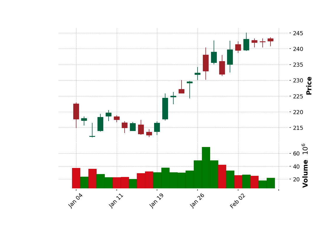
From a candlestick chart(zoom the graph), a green candlestick indicates a day where the closing price was higher than the open(Gain), while a red candlestick indicates a day where the open was higher than the close (Loss). The wicks indicate the high and the low, and the body the open and close (hue is used to determine which end of the body is open and which the close). You can follow the instruction from the following example to change the color. You need to pass your own style to the plot function. And as I said previously, a user can use Candlestick charts for technical analysis and use them to make trading decisions, depending on the candles' shape, color, and position. We will not cover a technical analysis in this example.
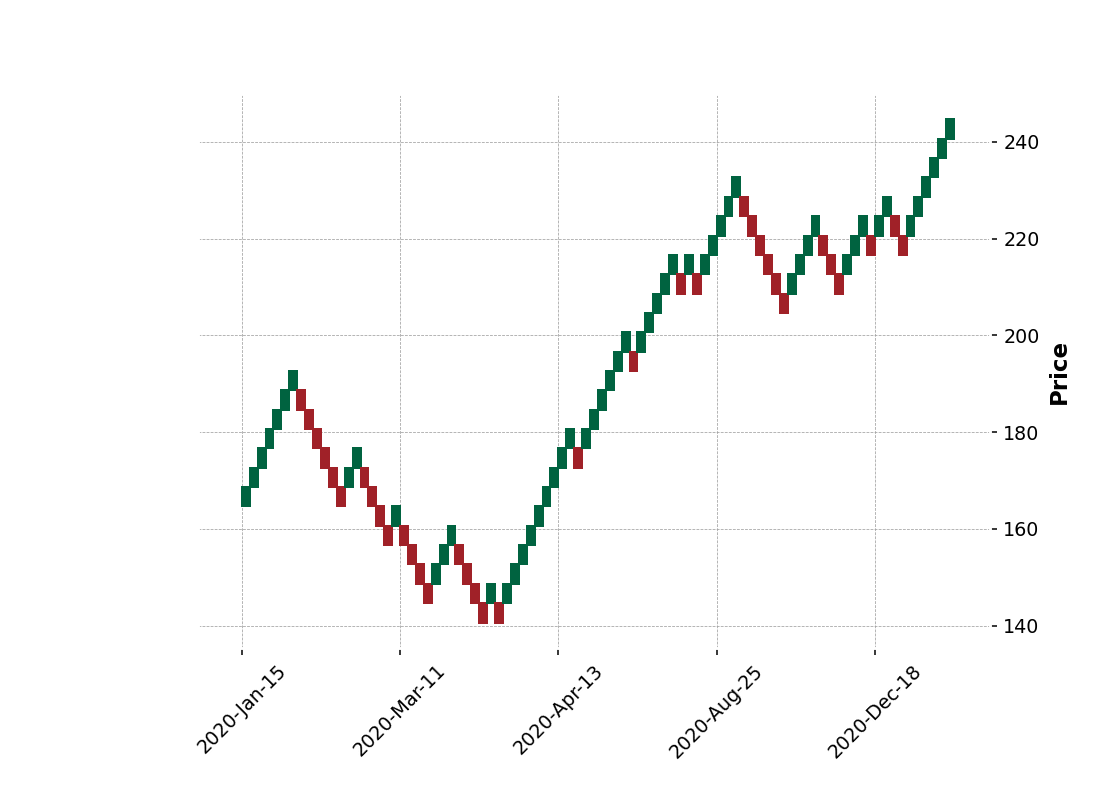
Plot OHLC chart
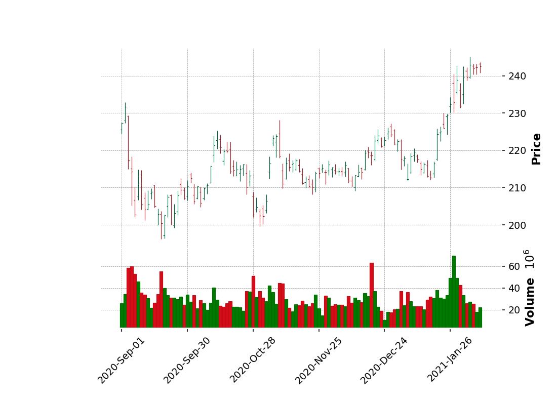
An OHLC chart is a type of bar chart that shows open, high, low, and closing prices for each period. OHLC charts are useful since they show the four major data points over a period, with the closing price being considered the most important by many traders. The chart type is useful because it can show increasing or decreasing momentum. When the open and close are far apart, it shows strong momentum, and when they open and close are close together, it shows indecision or weak momentum. The high and low show the full price range of the period, useful in assessing volatility. There several patterns traders watch for on OHLC charts [8].
To plot the OHLC chart, you can just change the type to 'ohlc'. It's quite easy when using mplfinance.
mpf.plot(dfPlot.loc['2020-09-01':str(datetime.date.today()),:],type='ohlc',style='charles',volume=True)
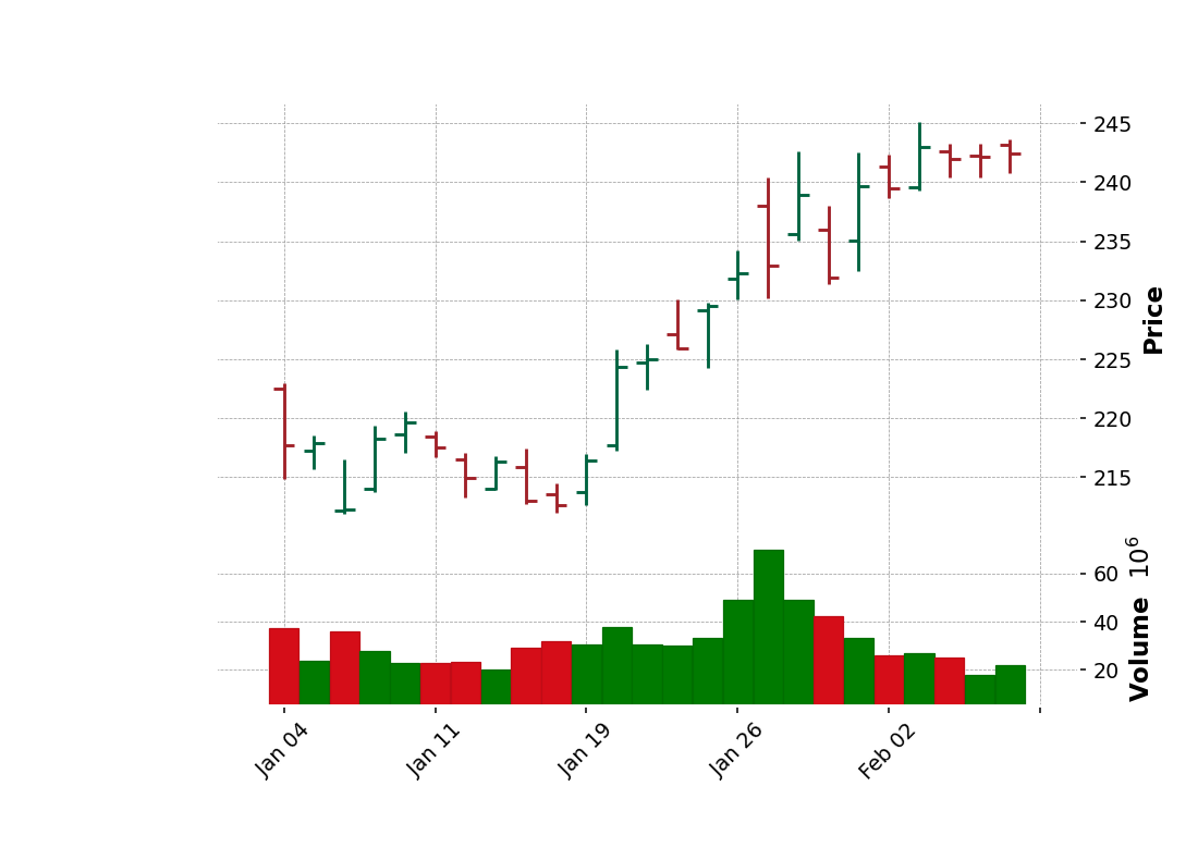
display(dfPlot)
mpf.plot(dfPlot.loc['2021-01-01':str(datetime.date.today()),:],type='ohlc',style='charles',volume=True)
Adding plots to the basic mplfinance plot()
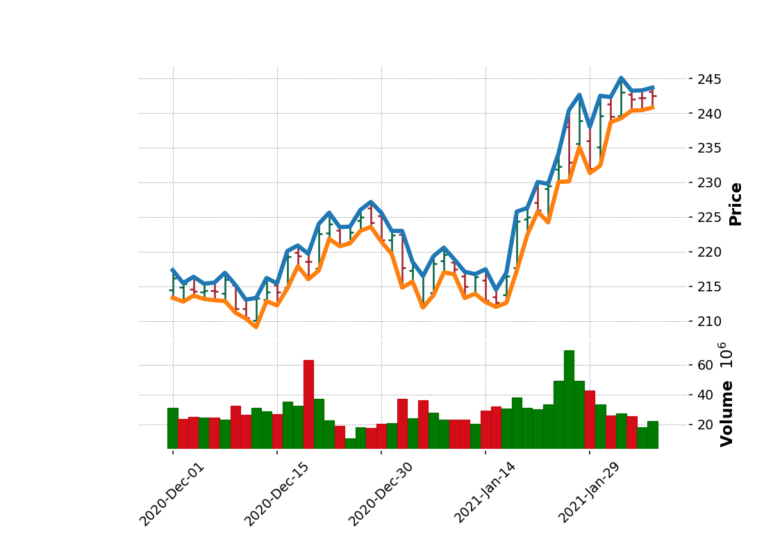
Sometimes you may want to plot additional data within the same figure as the basic OHLC or Candlestick plot. For example, you may want to add the results of a technical study or some additional market data.
This is done by passing information into the call to mplfinance.plot() using the addplot ("additional plot") keyword. I will show you a sample of the additional plots by adding a line plot for the data from columns High and Low to the original OHLC chart.
dfSubPlot = dfPlot.loc['2020-12-01':str(datetime.date.today()),:]
apdict = mpf.make_addplot(dfSubPlot[['High','Low']])
mpf.plot(dfSubPlot,type='ohlc',style='charles',volume=True,addplot=apdict)
Add Simple Moving Average to the Chart
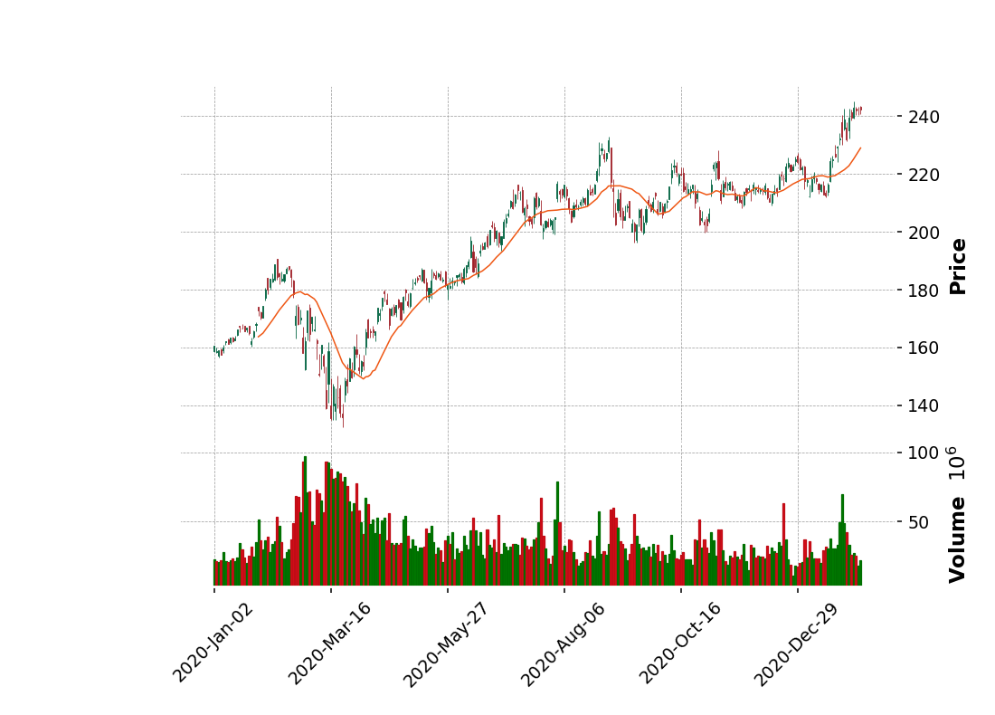
Next steps, we will add a moving average (MA) to the CandleStick chart. MA is widely used as the technical analysis indicator that helps smooth out price action by filtering out the “noise” from random short-term price fluctuations. It is a trend-following or lagging indicator because it is based on past prices. The two basic and commonly used moving averages are the simple moving average (SMA), the simple average of a security over a defined number of time periods, and the exponential moving average (EMA), giving greater weight to more recent prices. Note that this example will use only built-in MA provided by the mplfinance. The most common moving averages are to identify the trend direction and determine support and resistance levels.
Basically, mplfinance provides functionality for easily computing a moving average. The following codes creating a 20-day moving average from the price provided in the dataframe, and plotting it alongside the stock. Moving averages lag behind current price action because they are based on past prices; the longer the time period for the moving average, the greater the lag. Thus, a 200-day MA will have a much greater degree of lag than a 20-day MA because it contains prices for the past 200 days.
mpf.plot(dfPlot.loc[:str(datetime.date.today()),:],type='candle',style='charles',mav=(20),volume=True)
The length of the moving average to use depends on the trading objectives, with shorter moving averages used for short-term trading and longer-term moving averages more suited for long-term investors. The 50-day and 200-day MAs are widely followed by investors and traders, with breaks above and below this moving average considered important trading signals.
The following codes use to generated CandleStick charts with multiple periods of times for SMA (20-day,50-day,75-day, and 200-day).
mpf.plot(dfPlot.loc[:str(datetime.date.today()),:],type='candle',style='charles',mav=(20,60,75,200),volume=True)
Zoom the chart to display shorter period.
You can also calculate the moving average from your own method or algorithm using the original data from the dataframe and then add a subplot to the CandleStick charts using add plot like the previous sample of OHLC charts.
Generate Renko Chart
Based on the investopedia page, a Renko chart is a type of chart developed by the Japanese that is built using price movement rather than both price and standardized time intervals like most charts are. It is thought to be named after the Japanese word for bricks, "renga," since the chart looks like a bricks series. A new brick is created when the price moves a specified price amount, and each block is positioned at a 45-degree angle (up or down) to the prior brick. An up brick is typically colored white or green, while a down brick is typically colored black or red[7].
Renko charts filter out the noise and help traders more clearly see the trend since all smaller movements than the box size are filtered out.Renko charts typically only use closing prices based on the chart time frame chosen. For example, if using a weekly time frame, weekly closing prices will be used to construct the bricks[7].
mpf.plot(dfPlot,type='renko',style='charles',renko_params=dict(brick_size=4))
You can also watch the following video to summarize details about the RDP Library for Python we use in this article with a demo of the API usage.
Summary
This article explains RDP users' alternate choices to retrieve such kind of the End of Day price or intraday data from the Refinitiv Data Platform. This article provides a sample code to use RDP Library for python to retrieve the RDP Historical Pricing service's intraday data. And then show how to utilize the data with the 3rd party library such as the mplfinance to plot charts like the CandleStick, OHLC, and Renko chart for stock price technical analysis. Users can specify a different kind of interval and adjustment behavior using the RDP Library to retrieve more specific data and visualize the data on various charts. They can then use the charts to identify trading opportunities in price trends and patterns seen on charts.