Forward Looking Index Ratio Analysis

April 25,2022

Susan Cluzel

Caroline Andrade

Marian Kelly

Nick Zincone

Investment bankers, strategists, and analysts frequently need to pull historical forward valuation ratios for indices, including Enterprise Value (EV) multiples that don't exist in our IBES aggregate data sets. Using Jupyter and Python, the following article outlines an algorithm to overcome the limitations of accessing Refinitiv content through legacy Excel COM APIs to create aggregates based on underlying constituents, thus addressing key performance, methodology, and the use of historical constituents challenges.

The algorithm focuses on creating aggregates for a specified index based on underlying constituents' data over a selected time frame, and all company-level data for CY1, CY2, and CY3 periods are calendarized to a December year-end prior to aggregation. The challenges when pulling "rolling" calendar periods using the capabilities within Excel is greatly simplified using the power of Python and our desktop APIs.

As a comparison metric, the code segments also provide the ability to pull historical time series estimates valuation multiples for a specified company and chart the comparison against the calculated index benchmark.

***Note: for indices, a direct license with the index provider may be required to pull constituents' data.

Getting Started

To get started, we will need to import the Eikon Data API responsible for pulling measures driving the analysis for our ratios. In addition, we'll include a convenient UI to enable the user to choose input parameters driving results. As part of our analysis, we'll need to manipulate the data and graph a comparison chart to observe the performance measures over time.

    	
            # Data Library
import eikon as ek
ek.set_app_key('DEFAULT_CODE_BOOK_APP_KEY')
 
# Standard Python modules for data collection and manipulation
import pandas as pd
import numpy as np
import datetime as dt
from datetime import date 
from datetime import datetime
import dateutil.relativedelta
from dateutil.relativedelta import relativedelta, FR
 
# UI display widgets
import ipywidgets as widgets
from ipywidgets import Box
 
# Graphing libraries
import plotly.express as px #the plotly libraries for visualization and UI
import plotly.graph_objects as go
 
# Progress bar
from tqdm.notebook import tqdm, trange

The following example notebook demonstrates data access within the desktop, whether Eikon or Refinitiv Workspace. The notebook can be loaded in either Refinitiv's fully hosted Python environment called CodeBook or within your own Jupyter environment. Above, you will see the standard CODEBOOK APP Key. If the choice is to run outside of CodeBook, you will need to replace the key with a key of your own from the APP KEY GENERATOR.

Process Workflow

The following workflow outlines concrete steps involved in generating our data analysis. The steps have been intentionally broken out into well-defined segments for the purposes of reusability as well as a basis for understanding the processing details.

Index Calculations
The Index calculations phase involves the capture and calculation of index ratios used as the basis for our benchmark comparison. The following steps are outlined:
- Capture input parameters
  A UI is presented to allow the capture of the details related to our index including the estimates financial period.
- Retrieve, prepare and chart the data
  Based on the input details, derive the data points from Refinitiv using the data APIs available. The extraction and calculation of data points involve a number of steps, including the capture of index constituents over time. A chart is presented providing a visual of the index over the specified time.
Company Calculations
With our Index analysis prepared, we can use this as our benchmark to compare against any chosen company. The Company calculations phase involves the capture and preparations of the select multiple for our company. The following steps are outlined:
- Capture input parameters
  A UI is presented to allow the capture of the details related to our company including the estimates financial period.
- Retrieve, prepare and chart the data
  Calculate the EV multiple creating a time-series representation based on the date range specified for our benchmark.
Analysis
Finally, combine and chart the data sets captured to analyze how our chosen company is performing against our benchmark.

Common functions

In preparation for our analysis, the following common functions have been defined as reusable modules across the workflow.

    	
            # Based on the selected period and date, convert to a period value recognized by the back-end data engine
period_table = {'CY1': lambda yr : f'CY{yr}',
                'CY2': lambda yr : f'CY{yr+1}',
                'CY3': lambda yr : f'CY{yr+2}'
               }
def define_period(period, dt):
    year = int(dt.strftime("%Y"))
    return period_table[period](year) if period in period_table else period

    	
            # Based on the selected frequency, retrieve the relative increment value for our date period
def increment_period(frequency):
    if frequency == 'Weekly':
        return relativedelta(weeks=1, weekday=FR)
    
    if frequency == 'Monthly':
        return relativedelta(months=1, day=31)
    
    return relativedelta(months=3, day=31)

    	
            # Convenience routine to capture the number of iterations within our progress bar
def progress_bar_cnt(start, end, freq):
    cnt = 0
    while start <= end:
        start += increment_period(freq)
        cnt = cnt+1
        
    return cnt

1 - Index Calculations:

Calculate the selected multiple for historical constituents for the specified index as of each historical date
Remove constituent duplicates in the case of multiple share classes for one company included within an index
Remove rows if either EV or estimate is NA to ensure a consistent universe in numerator and denominator
Exclude companies with negative estimates values
Divide the resulting sum of estimates into a sum of EVs for weighted values

EV multiple is calculated one date at a time and added to a collection to create the resulting time series for further analysis, such as charting and export. Calculations for EV multiples one date at a time are necessary for both of the following reasons:

Index constituents change over time
Calendar year financial periods need to "roll". i.e. CY1, CY2, and CY3 need to be relative to the calculation date.

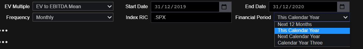
Index UI widgets

Capture the index parameters used to build our analysis:

    	
            measSelect = widgets.Dropdown(
    options = [('EV to EBITDA Mean','TR.EBITDAMean'), ('EV to Revenue Mean','TR.RevenueMean'), 
               ('EV to Free Cash Flow Mean','TR.FCFMean')],
    value = 'TR.EBITDAMean',
    description = 'EV Multiple'
)
 
start = widgets.DatePicker(
    value = datetime(2019, 12, 31).date(),
    description='Start Date'
)
 
end = widgets.DatePicker(
    value = datetime(2020, 12, 31).date(),
    description='End Date'
)
 
frqSelect = widgets.Dropdown(
    options = ['Weekly', 'Monthly', 'Quarterly'],
    value = 'Monthly',
    description = 'Frequency'
)
 
indSelect = widgets.Text(
    value='.SPX',
    placeholder='Enter RIC',
    description='Index RIC'
)
 
perSelect = widgets.Dropdown(
    options = [('Next 12 Months', 'NTM'), ('This Calendar Year','CY1'), 
               ('Next Calendar Year', 'CY2'), ('Calendar Year Three', 'CY3')],
    value = 'CY1',
    description = 'Financial Period',
    style = {'description_width': 'initial'}
)
 
items =[measSelect, start, end, frqSelect, indSelect, perSelect]
box = Box(children = items)
box

Retrieve and prepare the Index data

    	
            # define chain RIC for index 
Index = f'0#{indSelect.value}'   
 
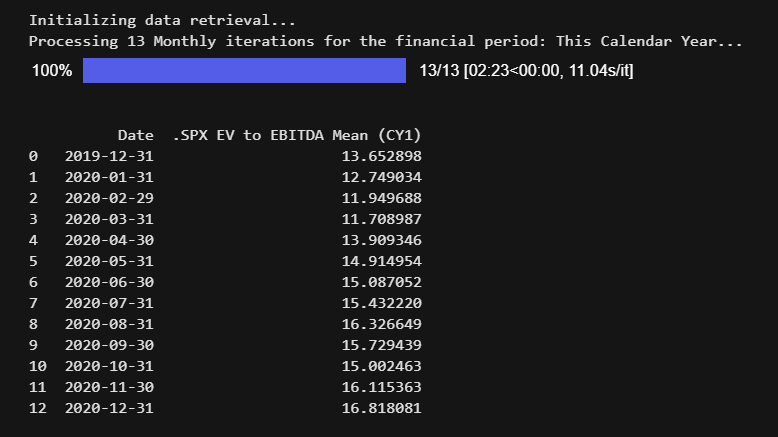
print("Initializing data retrieval...")
    
# Retrieve the currency for the index
index_curn, err = ek.get_data(Index,'TR.PriceClose.currency')
if err is None and end.value > start.value:
    Curn = index_curn.iloc[0,1]
 
    # Define the estimates measure for each constituent based on user input
    EstMeasure = measSelect.value
 
    # define label based on user input for data transparency. used in outputs, including 
    # dataframe viewing, charing and data export
    I_colLabel = f'{indSelect.value} {measSelect.label} ({perSelect.value})'
 
    #create empty dataframe to populate results
    index_data = pd.DataFrame(columns=['Date', I_colLabel])
 
    # define start date value based on user input and parameters for date frequency options
    d = start.value 
    
    # Based on the date range and the chosen frequency, determine the number of requests 
    # required to build out the data set
    iterations = progress_bar_cnt(start.value, end.value, frqSelect.value)
    print(f'Processing {iterations} {frqSelect.label} iterations for the financial period: {perSelect.label}...')
    for i in trange(iterations):
        
        # define absolute CY period for each date
        fperiod = define_period(perSelect.value, d)
        
        # Retrieve the index constuents based on the time period...
        constituents, err = ek.get_data(
            instruments = f'{Index}({d})',
            fields = ['TR.RIC',
             'TR.CommonName',
             f'TR.EV(sdate={d}, curn={Curn})',
             f'{EstMeasure}(Period={fperiod},sdate={d},Methodology=weightedannualblend, curn={Curn})',
             'TR.OrganizationID'])
 
        if err is None:
            constituents.rename(columns={ constituents.columns[4]: EstMeasure }, inplace = True)
 
             # exclude duplicate companies within index
            constituents.drop_duplicates(subset='Organization PermID', keep='first', 
                                         inplace=True, ignore_index=False)
            
             # exclude companies if EV or EBITDA is not available
            constituents.dropna(subset=[EstMeasure, 'Enterprise Value (Daily Time Series)'], inplace=True)
            
             # exclude companies when estimate is negative 
            constituents = constituents[constituents[EstMeasure].values > 0]
            
            # Finally, calculate the multiple
            EV_Multiple = constituents['Enterprise Value (Daily Time Series)'].sum() / constituents[EstMeasure].sum()
 
            result = [d, EV_Multiple]
            a_series = pd.Series(result, index = index_data.columns) # convert list object to DataFrame
            index_data = index_data.append(a_series, ignore_index = True)
 
            # Retrieve the next date within our period
            d += increment_period(frqSelect.value)
        else:
            print(f"Failed to retrieve constituents for Index: {Index}({d})")
            print(err)
            break
 
    # Display the resulting time series data - provides a visual for data validation
    print(index_data)
else:
    errMsg = "Invalid date(s) specified" if err is None else f'Index {Index} - {err}'
    print(f"Failed to retrieve Currency details - {errMsg}")

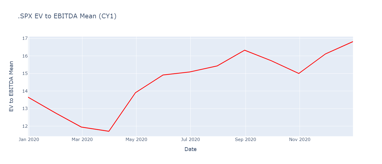
Prepare and chart the index data

    	
            # time series dates are converted to a date format for charting
index_data['Date'] = pd.to_datetime(index_data['Date'])
 
# Index data chart
fig = px.line(index_data, x='Date', y=I_colLabel, title= I_colLabel)
fig.update_yaxes(title_text=measSelect.label)
fig.update_traces(line_color='#FF0000')
fig.show()

2 - Company Calculations:

EV multiple is pulled one date at a time to create the resulting time series for analysis. Calculations for EV multiples one date at a time are necessary in case the user chooses a calendar year financial period for the estimates data to compare companies with different fiscal year ends. Fiscal year financial periods are also input options.

Company UI widgets

Capture the company parameters used to build our analysis:

    	
            multSelect = widgets.Dropdown(
    options = [('EV to EBITDA Mean','TR.EVtoEBITDAMean'), ('EV to Revenue Mean','TR.EVtoRevenueMean'), 
               ('EV to Free Cash Flow Mean','TR.EVtoFCFMean')],
    value = 'TR.EVtoEBITDAMean',
    description = 'EV Multiple'
)
 
ricSelect = widgets.Text(
    value='IBM',
    placeholder='Enter RIC',
    description='Company RIC',
    style = {'description_width': 'initial'}
)
 
Co_perSelect = widgets.Dropdown(
    options = [('Next 12 Months', 'NTM'), ('This Calendar Year','CY1'), 
               ('Next Calendar Year', 'CY2'), ('Calendar Year Three', 'CY3'),
               ('This Fiscal Year','FY1'),  ('Next Fiscal Year', 'FY2'), 
               ('Fiscal Year Three', 'FY3')
              ],
    value = 'CY1',
    description = 'Financial Period',
    style = {'description_width': 'initial'}
)
 
items =[multSelect, ricSelect, Co_perSelect]
box = Box(children = items)
box

Retrieve and prepare the Company data

    	
            err = None
EstMeasure = multSelect.value
 
# Create dataframe for resultsing time series data
company_data = pd.DataFrame()
 
# Define start date value based on user input and parameters for date frequency options
d = start.value 
    
# Based on the date range and the chosen frequency, determine the number of requests required
# to build out the data set
iterations = progress_bar_cnt(start.value, end.value, frqSelect.value)
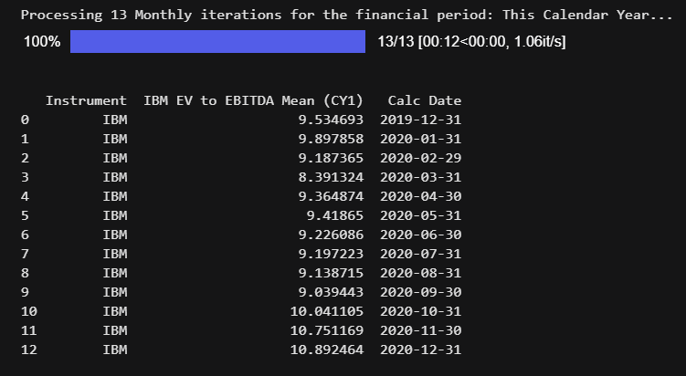
print(f'Processing {iterations} {frqSelect.label} iterations for the financial period: {Co_perSelect.label}...')
for i in trange(iterations):
    # define absolute CY period for each date
    fperiod = define_period(Co_perSelect.value, d)
    
    CoEV_Multiple, err = ek.get_data(
        instruments = ricSelect.value,
        fields = [f'{EstMeasure}(Period={fperiod},sdate={d},Methodology=weightedannualblend)',
                  f'{EstMeasure}(Period={fperiod},sdate={d}).CalcDate'])    
  
    if err is None:
        company_data=company_data.append(CoEV_Multiple, ignore_index=True)
    
        # Retrieve the next date within our period
        d += increment_period(frqSelect.value)  
    else:
        print(f"Failed to retrieve data for company: {ricSelect.value})")
        print(err)
        break        
 
if err is None:   
    # Define label based on user input for data transparency. used in outputs, 
    # including dataframe viewing, charting and data export
    C_colLabel = f'{ricSelect.value} {multSelect.label} ({Co_perSelect.value})'
    company_data.rename(columns={ company_data.columns[1]: C_colLabel }, inplace = True)
    
    print(company_data) # Print resulting time series to assist in data validation)

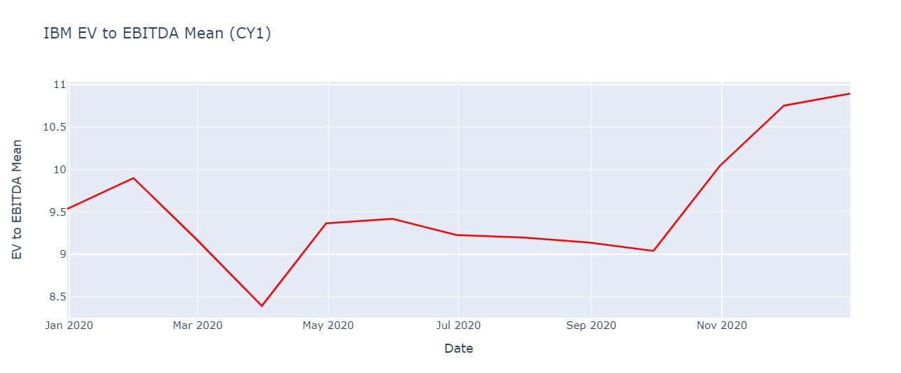
Prepare and chart the company data

    	
            # Normalize the company data set to ensure names and types are consistent for later analysis
company_data['Calc Date'] = pd.to_datetime(company_data['Calc Date'])
company_data.rename(columns={ 'Calc Date': 'Date' }, inplace = True)
company_data[C_colLabel] = company_data[C_colLabel].astype(float)
 
# Index data chart
fig = px.line(company_data, x='Date', y=C_colLabel, title= C_colLabel)
fig.update_yaxes(title_text=measSelect.label)
fig.update_traces(line_color='#FF0000')
fig.show()

3 - Analysis

Once our data sets have been normalized, we can combine the result sets to perform the analysis of comparing the selected company against our chosen benchmark (index).

    	
            # Merge company and index data...
chart_data = index_data.merge(company_data, how='inner', on='Date')
chart_data

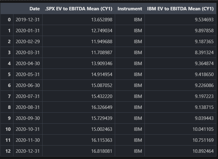
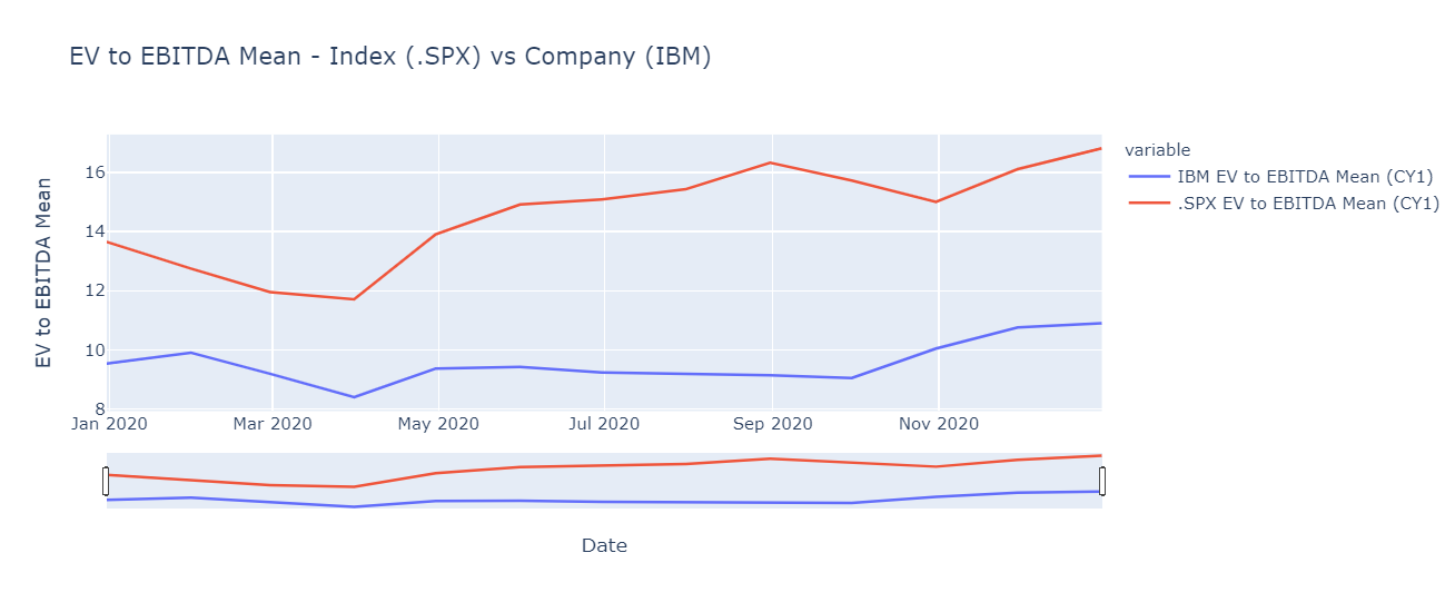
Chart index and company data

    	
            # Index and selected company chart
fig = px.line(chart_data,
             x="Date",
             y=[C_colLabel,I_colLabel],
             title=f'{multSelect.label} - Index ({indSelect.value}) vs Company ({ricSelect.value})')
fig.update_yaxes(title_text= multSelect.label)
fig.update_layout(xaxis_rangeslider_visible=True)
fig.show()

Additional Analysis

Once our data has been prepared, further analysis can be integrated with your own business workflows to be used in comps and valuation models. Whether ingesting the computed data frames within existing Python modules and importing the data set as import files, many options are available. For example, the following code segment exports our data set within Excel:

    	
            with pd.ExcelWriter('EV Multiples.xlsx') as writer:
    index_data.to_excel(writer, sheet_name='Index EV Multiple',index=False)
    company_data.to_excel(writer, sheet_name='Company Multiple', index=False)

Conclusion

In this article, we have used the power of python along with the extensive data from Refinitiv to create valuation ratios for indices that can be used to make comparisons across markets, sectors, and time and as a benchmark to value companies.

We have used a bottom-up approach to calculate an index aggregate based on underlying constituents' data. Important concepts demonstrated are that of a chain RIC to pull index constituents as of a given point in time and a method of calculating a time series with a rolling calendar year financial period.

And finally, using Jupyter and Python, we have been able to overcome the limitations of accessing Refinitiv content through legacy Excel COM APIs.

Source Code

GitHub - Python Jupyter Notebook

Related APIs

Eikon Data API

Articles

Developer Tools

Use Cases

Upcoming Events

Past Events

About Us