
In this article, we look at how one may choose an optimal SARIMA model by selecting the one with lowest in-sample errors. We also look into how one may use both Eikon and Datastream data together, as well as statistical concepts of stationarity and differencing among others. We also investigate and compare models only using comparative months (e.g.: Jan. with Jan., Feb. with Feb., etc.). You may see the Webinar recording at the end.
We find that the optimal model is a SARIMA(5,0,4)(4,0,0)$_{12}$.
To do so we look at (i) how one may check for stationarity graphically and via (ADF, KPSS & PP) test statistics, (ii) differencing, (iii) ex-ante (before modelling) parameter identification via autocorrelation & partial autocorrelation functions, (iv) the difference between Autoregressive Moving Average (ARMA) & Seasonal Integrated ARMA (SARIMA) models, (v) ex-post (after modelling) parameter identification via information criteria and mean of absolute & squared errors (as well as the use of Python's 'pickle' library), (vi) how one may choose an optimal model specification - reducing errors, (vii) recursive one-step-ahead out-of-sample forecasts, and finally (iix) corresponding month models before concluding.
As a precursor to ARMA modelling, the reader is advised to read 'Information Demand and Stock Return Predictability (Coded in R): Part 2: Econometric Modelling of Non-Linear Variances' - an article without coding that looks into our methods of modelling.
Contents
- What are SARIMA Models?
- Get to Coding
- Data Sets
- Stationarity
- Modelling
- Conclusion
- Webinar Recording
- References
What are SARIMA Models?
Seasonal AutoRegressive Integrated Moving Average (SARIMA) models are best explained in a separate article. "Time Series Forecasting with SARIMA in Python" is great at showing both the mathematics and fundamental Python basics at play below. I would suggest reading this article 1st that goes through the slightly simpler ARMA model. The only difference is the inclusion of the seasonal factor in:
SARIMA(5,0,4)(4,0,0)$_{12}$:
$$\begin{align} y_t &= c + \sum_{j=1}^{5} \phi_j y_{t-j} + \sum_{i=1}^{4} \psi_i \epsilon_{t-i} + \sum_{J=1}^{4} \Phi_i y_{t-(J*12)} \\ &= c + \phi_1 y_{t-1} + \phi_2 y_{t-2} + \phi_3 y_{t-3} + \phi_4 y_{t-4} + \phi_5 y_{t-5} + \psi_1 \epsilon_{t-1} + \psi_2 \epsilon_{t-2} + \psi_3 \epsilon_{t-3} + \psi_4 \epsilon_{t-4} + \Phi_1 y_{t-(1*12)} + \Phi_2 y_{t-(2*12)} + \Phi_3 y_{t-(3*12)} + \Phi_4 y_{t-(4*12)} \\ &= c + \phi_1 y_{t-1} + \phi_2 y_{t-2} + \phi_3 y_{t-3} + \phi_4 y_{t-4} + \phi_5 y_{t-5} + \psi_1 \epsilon_{t-1} + \psi_2 \epsilon_{t-2} + \psi_3 \epsilon_{t-3} + \psi_4 \epsilon_{t-4} + \Phi_1 y_{t-12} + \Phi_2 y_{t-24} + \Phi_3 y_{t-36} + \Phi_4 y_{t-48} \end{align}$$
In our study, we will also use exogenous variables ($x_t$'s) too such that - for a model with $m$ exogenous variables with potentially different $r_k$ lags each:
$ y_t = c + \sum_{j=1}^{5} \phi_j y_{t-j} + \sum_{i=1}^{4} \psi_i \epsilon_{t-i} + \sum_{J=1}^{4} \Phi_i y_{t-(J*12)} + \sum_{k=1}^{m} \left( \sum_{n= 1}^{r_k} \beta_{k,n} x_{k , t-{r_k}} \right)$
Get to Coding 
Development Tools & Resources
The example code demonstrating the use case is based on the following development tools and resources:
- Refinitiv's DataStream Web Services (DSWS): Access to DataStream data. A DataStream or Refinitiv Workspace IDentification (ID) will be needed to run the code below.
- Refinitiv's Eikon API: To access Eikon data. An Eikon API key will be needed to use this API.
Import Libraries
We need to gather our data. Since Refinitiv's DataStream Web Services (DSWS) allows for access to ESG data covering nearly 70% of global market cap and over 400 metrics, naturally it is more than appropriate. We can access DSWS via the Python library "DatastreamDSWS" that can be installed simply by using pip install.
import DatastreamDSWS as dsws
# We can use our Refinitiv's Datastream Web Socket (DSWS) API keys that allows us to be identified by Refinitiv's back-end services and enables us to request (and fetch) data: Credentials are placed in a text file so that it may be used in this code without showing it itself.
(dsws_username, dsws_password) = (open("Datastream_username.txt","r"),
open("Datastream_password.txt","r"))
ds = dsws.Datastream(username = str(dsws_username.read()),
password = str(dsws_password.read()))
# It is best to close the files we opened in order to make sure that we don't stop any other services/programs from accessing them if they need to.
dsws_username.close()
dsws_password.close()
# # Alternatively one can use the following:
# import getpass
# dsusername = input()
# dspassword = getpass.getpass()
# ds = dsws.Datastream(username = dsusername, password = dspassword)
We use Refinitiv's Eikon Python Application Programming Interface (API) to access financial data such as Clc1. We can access it via the Python library "eikon" that can be installed simply by using pip install.
import eikon as ek
# The key is placed in a text file so that it may be used in this code without showing it itself:
eikon_key = open("eikon.txt","r")
ek.set_app_key(str(eikon_key.read()))
# It is best to close the files we opened in order to make sure that we don't stop any other services/programs from accessing them if they need to:
eikon_key.close()
import numpy as np
import pandas as pd
import pickle # need to ' pip install pickle-mixin '. This library is native to Python and therefore doesn't have a version of its own.
from datetime import datetime, timedelta # ' datetime ' is native to Python and therefore doesn't have a version of its own.
# Import the relevant plotting libraries:
import plotly # Needed to show plots in line in Notebook.
from plotly.offline import init_notebook_mode, iplot
init_notebook_mode(connected = False) # Initialize plotly.js in the browser if it hasn't been loaded into the Document Object Model (DOM) yet.
import cufflinks, seaborn # Needed to show plots in line in Notebook.
cufflinks.go_offline() # plotly & cufflinks are online platforms but we want to stay offline.
for i,j in zip([ek, np, pd, plotly, cufflinks, seaborn],
["eikon", "numpy", "pandas", "plotly", "cufflinks", "seaborn"]):
print("The library '" + j + "' in this notebook is version " + i.__version__)
The library 'eikon' in this notebook is version 1.1.8
The library 'numpy' in this notebook is version 1.18.2
The library 'pandas' in this notebook is version 1.2.4
The library 'plotly' in this notebook is version 4.14.3
The library 'cufflinks' in this notebook is version 0.17.3
The library 'seaborn' in this notebook is version 0.11.1
Data-sets
Dependent variables (Y):
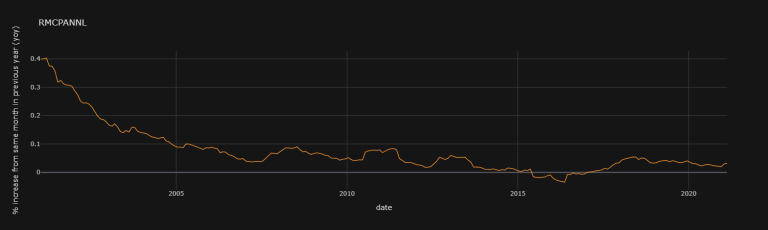
RMCPANNL: Romania, Consumer Prices, by Commodity, All Items, Total, Change y/y
Annual inflation rate – the increase (in percentage term) in consumer prices in one month of the current year compared to the same month of the previous year. This rate is calculated as a ratio, expressed as a percentage, between the price index of one month of the current year and that of the same month of the previous year, calculated against the same base, from which 100 is subtracted.
This data-set will be differenced once to be stationary.
RMCONPRCF
Independent / Explanatory variables (X):
Each of the following datasetes can be used in 'raw' (id est (i.e.): without changing the data retrieved from Datastream) or adjusted like RMCPANNL (i.e.: looking at that metric's increase in one month compared to the same month of the previous year and then differenced once to be stationary) each defined as 'raw' or 'yoy' variables respectively.
- RMUNPTOTP: Romania, Unemployed, Overall, Registered.
- CLc1: 'CLc1 NYMEX Light Sweet Crude Oil (WTI) Electronic Energy Future Continuation 1' on eikon (which we will use) and 'NYMEX - Light Crude Oil TRC1' on Datastream: Crude oil prices from the US market's NYMEX (New York Mercantile Exchange).
- RMXRUSD.: Romania, New Romanian Leu Per US Dollar, RON: Foreign Exchange (FX) rate of 1USD to 1Leu.
- RMXREUR.: Romania, New Romanian Leu Per Euro, RON: Foreign Exchange (FX) rate of 1EUR to 1Leu.
- RMGOVBALA: Romania, Deficit / Surplus, GFS2001, Total (New Methodology Since January 2006), Cumulative, RON: Romanian Government's National Debt level. If this value is positive, it indicates a surplus; if it is negative, it indicates a deficit.
Due to popular demand, we decided not to use Consumer Prices (Romania, Consumer Prices, by Commodity, All Items, Total, Index, Corresponding Period of the Previous Year = 100) as a dependent variable, but RMCPANNL instead.
Collecting Datastream Data
We can go ahead and collect our data from Datastream:
df = ds.get_data(tickers = "RMCPANNL,RMUNPTOTP,RMXRUSD.,RMXREUR.,RMGOVBALA", # be carefulnot to put spaces in between elements here, or else these spaces will be included in column names.
fields = "X",
start = '2000-01-01',
end = '2021-04-06',
freq = 'M')
Note that RMCPANNL's values are percentages, we thus ought to divide it by 100 to get proper fractions:
df["RMCPANNL", "X"] = df["RMCPANNL"]["X"]/100
Let's have a look at our Pandas data-frame ' df '
df
| Instrument | RMCPANNL | RMUNPTOTP | RMXRUSD. | RMXREUR. | RMGOVBALA |
|---|---|---|---|---|---|
| Field | X | X | X | X | X |
| Dates | |||||
| 2000-01-15 | 0.5680 | 1175.0 | 1.84 | 1.8636 | -162.8 |
| 2000-02-15 | 0.5570 | 1196.6 | 1.87 | 1.8421 | -461.9 |
| 2000-03-15 | 0.4900 | 1166.7 | 1.92 | 1.8538 | -826.0 |
| 2000-04-15 | 0.4890 | 1139.2 | 1.98 | 1.8713 | -1210.9 |
| 2000-05-15 | 0.4400 | 1097.4 | 2.04 | 1.8507 | -1367.8 |
| ... | ... | ... | ... | ... | ... |
| 2020-12-15 | 0.0206 | 296.1 | 4.00 | 4.8707 | -105906.6 |
| 2021-01-15 | 0.0299 | 292.2 | 4.00 | 4.8728 | -112.3 |
| 2021-02-15 | 0.0316 | 293.5 | 4.03 | 4.8741 | -8430.8 |
| 2021-03-15 | 0.0305 | NaN | 4.11 | 4.8878 | NaN |
| 2021-04-15 | NaN | NaN | NaN | NaN | NaN |
256 rows × 5 columns
Note on timing: I aim to make this article as realistic as possible, putting myself in the shoes of a professional using this workflow to predict inflation. I do not expect our SARIMA models to perform particularly well, mainly because we did not do extensive research on the best exogenous variables to use - I leave that to you to decide. But while I do not expect this model to perform well, the workflow ought to be at its best. To use it optimally, please try to use exogenous variables (such as RMXRUSD.) as soon as their monthly values are released. It is possible for the values as of the - 15th of the month - of one variable to be published at another time to another (exempli gratia (e.g.): values for RMXRUSD. and RMGOVBALA could be published on the 20th and 25th of the month respectively, even though they are both representing values for the 15th of the month).
The 'X' is the default value for each of the items we requested. Let's change those with relevant value names:
df.columns = pd.MultiIndex.from_tuples(
[('RMCPANNL', 'yoy'), # yoy will be the increase in one month compared to the same month of the previous year
('RMUNPTOTP', 'raw'),
('RMXRUSD.', 'raw'),
('RMXREUR.', 'raw'),
('RMGOVBALA', 'raw')],
names=['Instrument', 'Field'])
CLc1, err = ek.get_data(
instruments = "CLc1",
fields = ["TR.CLOSEPRICE.timestamp",
"TR.CLOSEPRICE",
"MAVG(TR.CLOSEPRICE,-29)"],
parameters = {'SDate': '1999-01-01', # We want to start 1 year earlier because we're about to take moving averages which makes us loose degrees of freedom.
'EDate': str(datetime.today())[:10], # ' df.index[-1] ' picks the last date in our previously defined data-frame ' df '. You may want to use 'str(datetime.today())[:10]'.
'FRQ': 'D'})
CLc1
| Instrument | Timestamp | Close Price | MAVG(TR.CLOSEPRICE,-29) | |
| 0 | CLc1 | 1999-01-01T00:00:00Z | <NA> | 11.5477 |
| 1 | CLc1 | 1999-01-04T00:00:00Z | 12.36 | 11.5667 |
| 2 | CLc1 | 1999-01-05T00:00:00Z | 12 | 11.611 |
| 3 | CLc1 | 1999-01-06T00:00:00Z | 12.85 | 11.646 |
| 4 | CLc1 | 1999-01-07T00:00:00Z | 13.05 | 11.6833 |
| ... | ... | ... | ... | ... |
| 5592 | CLc1 | 2021-04-13T00:00:00Z | 60.45 | 61.6431 |
| 5593 | CLc1 | 2021-04-14T00:00:00Z | 62.75 | <NA> |
| 5594 | CLc1 | 2021-04-15T00:00:00Z | 63.32 | <NA> |
| 5595 | CLc1 | 2021-04-16T00:00:00Z | 63.07 | <NA> |
| 5596 | CLc1 | 2021-04-19T00:00:00Z | <NA> | <NA> |
5597 rows × 4 columns
But note that the last few moving average data points are NaN. Just in case these last few days are useful, let's make our own moving average:
# This takes the moving average of the last 30 datapoints, not the last 30 days (since not all of the last 30 days might have been trading days with price data).
CLc1["CLc1 30D Moving Average"] = CLc1["Close Price"].dropna().rolling(30).mean()
# Let's remove the ' MAVG(TR.CLOSEPRICE,-29) ' column, it was only there to display the issue outlined.
CLc1.drop('MAVG(TR.CLOSEPRICE,-29)', axis = 1, inplace = True)
CLc1 # Let's have a look at our data-frame now.
| Instrument | Timestamp | Close Price | CLc1 30D Moving Average | |
| 0 | CLc1 | 1999-01-01T00:00:00Z | <NA> | NaN |
| 1 | CLc1 | 1999-01-04T00:00:00Z | 12.36 | NaN |
| 2 | CLc1 | 1999-01-05T00:00:00Z | 12 | NaN |
| 3 | CLc1 | 1999-01-06T00:00:00Z | 12.85 | NaN |
| 4 | CLc1 | 1999-01-07T00:00:00Z | 13.05 | NaN |
| ... | ... | ... | ... | ... |
| 5592 | CLc1 | 2021-04-13T00:00:00Z | 60.45 | 61.645 |
| 5593 | CLc1 | 2021-04-14T00:00:00Z | 62.75 | 61.7543 |
| 5594 | CLc1 | 2021-04-15T00:00:00Z | 63.32 | 61.8297 |
| 5595 | CLc1 | 2021-04-16T00:00:00Z | 63.07 | 61.7977 |
| 5596 | CLc1 | 2021-04-19T00:00:00Z | <NA> | NaN |
5597 rows × 4 columns
Joining the Datastream and Eikon data-frames together
Now, if we want to combine the data from df and CLc1, we may want to do so joining the two data-frames on their dates; but one may notice that CLc1's Timestamp and df's index (Dates) portray time in different ways:
CLc1.Timestamp[0] # Note that ' CLc1.Timestamp ' is the same as CLc1["Timestamp"]
'1999-01-01T00:00:00Z'
df.index[0]
'2000-01-15'
To harmonize the two, I will use df's way:
'2000-01-31T00:00:00Z'[0:10]
'2000-01-31'
CLc1.index = [i[0:10] for i in CLc1.Timestamp]
CLc1
| Instrument | Timestamp | Close Price | CLc1 30D Moving Average | |
| 01/01/1999 | CLc1 | 1999-01-01T00:00:00Z | <NA> | NaN |
| 04/01/1999 | CLc1 | 1999-01-04T00:00:00Z | 12.36 | NaN |
| 05/01/1999 | CLc1 | 1999-01-05T00:00:00Z | 12 | NaN |
| 06/01/1999 | CLc1 | 1999-01-06T00:00:00Z | 12.85 | NaN |
| 07/01/1999 | CLc1 | 1999-01-07T00:00:00Z | 13.05 | NaN |
| ... | ... | ... | ... | ... |
| 13/04/2021 | CLc1 | 2021-04-13T00:00:00Z | 60.45 | 61.645 |
| 14/04/2021 | CLc1 | 2021-04-14T00:00:00Z | 62.75 | 61.7543 |
| 15/04/2021 | CLc1 | 2021-04-15T00:00:00Z | 63.32 | 61.8297 |
| 16/04/2021 | CLc1 | 2021-04-16T00:00:00Z | 63.07 | 61.7977 |
| 19/04/2021 | CLc1 | 2021-04-19T00:00:00Z | <NA> | NaN |
5597 rows × 4 columns
Now we are encountering the issue whereby the 15th of the month every month is not necessarily a trading day. But we want to normalise the two data-frames to have monthly data on the 15th of every month (since that's how Datastream returns data). What we can do is use CLc1 30D Moving Average on the 15th of every month and (if it's not available) we'll use the 14th's; if that's unavailable we'll use the 13th; and so on until a set limit - say the 12th of every month (repeating this process 3 times). This is what the function below does:
def Match_previous_days(df1, df2, common_day = 15, back = 3):
"""Match_previous_days Version 1.0:
This function compares two Pandas data-frames (df1 and df2, with monthly and daily
data respectively and dates in its index), and checks if any index from df1 is
missing in df2. If one for a day set in 'common_day' is missing, it changes it to
the previous day. It does so as many times as is set in 'back'.
It is created to ease the joining of Datastream API (DSWS) and Eikon API
retrieved Pandas data-frames (df1 and df2 respectively). E.g.:
Setting ' common_day ' to ' 15 ' and back to ' 3 ', our function will scan for
any row-name (called an index) in df1 for the 15th of the month that does not
appear in df2 and change any such index name to the 14th of the month (essentially
showing df2 data for the 14th of the month for those rows specifically as 15th of
the month). It can do it again for the 13th of the month, and then 12th; 3 times
in total (as specified in ' back ').
Parameters:
----------
df1: Pandas data-frame
A monthly data-frame from DSWS - or formatted similarly
(i.e.: with Multi-Index'ed columns, etc.).
df2: Pandas data-frame
A daily data-frame from eikon's API - or formatted
similarly - with one exception that its index is made of strings for dates in the
"yyyy-mm-dd" format.
common_day: int
The day of the month to start from. For an example, see 1st
paragraph above.
Default: common_day = 15
common_day: int
The number of times we are ready to run the procedure for. For an
example, see 1st paragraph above.
Default: back = 3
Dependencies:
----------
pandas 1.2.3
numpy 1.19.5
Examples:
--------
>>> import DatastreamDSWS as dsws
>>> ds = dsws.Datastream(username = "insert dsws username here", password = "insert dsws password here")
>>>
>>> import eikon as ek
>>> ek.set_app_key("insert eikon key here")
>>>
>>> df_1 = ds.get_data(tickers = "RMCPANNL,RMUNPTOTP,RMXRUSD.,RMXREUR.,RMGOVBALA", # be carefulnot to put spaces in between elements here, or else these spaces will be included in column names.
>>> fields = "X", start = '2000-01-01', freq = 'M')
>>>
>>> df_2, err = ek.get_data(instruments = "CLc1", fields = ["TR.CLOSEPRICE.timestamp", "TR.CLOSEPRICE"],
>>> parameters = {'SDate': '1999-01-01', # We want to start 1 year earlier because we're about to take moving averages which makes us loose degrees of freedom.
>>> 'EDate': str(datetime.today())[:10], # ' df_1.index[-1] ' picks the last date in our previously defined data-frame ' df_1 '. You may want to use 'str(datetime.today())[:10]'.
>>> 'FRQ': 'D'})
>>> df_2["CLc1 30D Moving Average"] = df_2["Close Price"].rolling(30).mean() # This takes the moving average of the last 30 datapoints, not the last 30 days (since not all of the last 30 days might have been trading days with price data).
>>> df_2.index = [i[0:10] for i in CLc1.Timestamp]
>>>
>>> Match_previous_days(df1 = df_1, df2 = df_2, common_day = 15, back = 3) # Note that this is the same as ' Match_previous_days(df1 = df_1, df2 = df_2) '.
"""
_common_day = "-" + "{:02d}".format(common_day)
df2_list = []
df2_df1_diff_index1 = []
df2_df1_diff_index2 = []
index_dictionary = []
df2_list.append(df2.copy())
for k in range(back):
if k > 0:
df2_list.append(df2_list[-1])
df2_df1_diff_index1.append(np.setdiff1d(
df1.index.tolist(),
df2_list[k][df2_list[k].index.str.contains(_common_day)].index.tolist()))
df2_df1_diff_index2.append([
i.replace("-15", "-" + "{:02d}".format(common_day - 1 - k)) # ' -1 ' because k starts at 0.
for i in df2_df1_diff_index1[k]])
index_dictionary.append({})
# display(index_dictionary[k])
for i,j in zip(df2_df1_diff_index2[k], df2_df1_diff_index1[k]):
index_dictionary[k][i] = j
# display(index_dictionary[k])
df2_list[k].rename(index = index_dictionary[k], inplace = True)
return df2_list[-1]
CLc1_of_interest0 = Match_previous_days(df1 = df, df2 = CLc1, common_day = 15, back = 4) # Applying the previously defined function.
CLc1_of_interest0.iloc[258:261]
| Instrument | Timestamp | Close Price | CLc1 30D Moving Average | |
| 13/01/2000 | CLc1 | 2000-01-13T00:00:00Z | 26.69 | 25.8317 |
| 15/01/2000 | CLc1 | 2000-01-14T00:00:00Z | 28 | 25.9453 |
| 18/01/2000 | CLc1 | 2000-01-18T00:00:00Z | 28.85 | 26.0753 |
As per the above, we can see the difference between the index and Timestamp in row 259, indicating that our function above worked.
CLc1_of_interest1 = CLc1_of_interest0[CLc1_of_interest0.index.str.contains("-15")] # We're only interested in the 15th of each month.
CLc1_of_interest = pd.DataFrame(
data = CLc1_of_interest1[
["Close Price", "CLc1 30D Moving Average"] # We're only interested in those two columns.
].values,
index = CLc1_of_interest1.index,
columns = pd.MultiIndex.from_tuples(
[('CLc1', 'Close Price'),
('CLc1', 'Close Price 30D Moving Average')]))
CLc1_of_interest
| CLc1 | ||
| Close Price | Close Price 30D Moving Average | |
| 15/01/1999 | 12.18 | NaN |
| 15/03/1999 | 14.46 | 12.6067 |
| 15/04/1999 | 16.88 | 15.5177 |
| 15/06/1999 | 18.54 | 17.667 |
| 15/07/1999 | 20.2 | 18.655 |
| ... | ... | ... |
| 15/12/2020 | 47.59 | 43.203 |
| 15/01/2021 | 52.04 | 48.7013 |
| 15/02/2021 | 59.73 | 53.606 |
| 15/03/2021 | 65.28 | 60.8053 |
| 15/04/2021 | 63.32 | 61.8297 |
265 rows × 2 columns
Now we can join our two data-frames:
df = pd.merge(df, CLc1_of_interest,
left_index = True,
right_index = True)
df
| Instrument | RMCPANNL | RMUNPTOTP | RMXRUSD. | RMXREUR. | RMGOVBALA | CLc1 |
|---|---|---|---|---|---|---|
| Field | yoy | raw | raw | raw | raw | Close Price |
| 2000-01-15 | 0.5680 | 1175.0 | 1.84 | 1.8636 | -162.8 | 28.0 |
| 2000-02-15 | 0.5570 | 1196.6 | 1.87 | 1.8421 | -461.9 | 30.03 |
| 2000-03-15 | 0.4900 | 1166.7 | 1.92 | 1.8538 | -826.0 | 30.65 |
| 2000-04-15 | 0.4890 | 1139.2 | 1.98 | 1.8713 | -1210.9 | 25.4 |
| 2000-05-15 | 0.4400 | 1097.4 | 2.04 | 1.8507 | -1367.8 | 29.97 |
| ... | ... | ... | ... | ... | ... | ... |
| 2020-12-15 | 0.0206 | 296.1 | 4.00 | 4.8707 | -105906.6 | 47.59 |
| 2021-01-15 | 0.0299 | 292.2 | 4.00 | 4.8728 | -112.3 | 52.04 |
| 2021-02-15 | 0.0316 | 293.5 | 4.03 | 4.8741 | -8430.8 | 59.73 |
| 2021-03-15 | 0.0305 | NaN | 4.11 | 4.8878 | NaN | 65.28 |
| 2021-04-15 | NaN | NaN | NaN | NaN | NaN | 63.32 |
256 rows × 7 columns
Now, we want comparable data, and RMCPANNL is the only series depicting the increase in one month compared to the same month of the previous year. So let's transform our other series to depict the data similarly:
df["RMUNPTOTP", "yoy"] = df["RMUNPTOTP"]["raw"].pct_change(periods = 12)
df["RMXRUSD.", "yoy"] = df["RMXRUSD."]["raw"].pct_change(periods = 12)
df["RMXRUSD.", "yoy"] = df["RMXRUSD."]["raw"].pct_change(periods = 12)
df["RMXREUR.", "yoy"] = df["RMXREUR."]["raw"].pct_change(periods = 12)
df["RMGOVBALA", "yoy"] = df["RMGOVBALA"]["raw"].pct_change(periods = 12)
df["CLc1", "yoy"] = df["CLc1"][
"Close Price 30D Moving Average"].pct_change(periods = 12)
df = df.sort_index(axis=1)
df = df.dropna()
df
| Instrument | CLc1 | RMCPANNL | RMGOVBALA | RMUNPTOTP | RMXREUR. | RMXRUSD. | ||||||
| Field | Close Price | Close Price 30D Moving Average | yoy | yoy | raw | yoy | raw | yoy | raw | yoy | raw | yoy |
| 15/01/2001 | 30.05 | 28.535 | 0.09981 | 0.399 | -306.1 | 0.88022 | 1032.9 | -0.1209 | 2.4646 | 0.32249 | 2.62 | 0.42391 |
| 15/02/2001 | 28.8 | 29.8113 | 0.07816 | 0.4 | -601.2 | 0.30158 | 1032.3 | -0.1373 | 2.4729 | 0.34244 | 2.68 | 0.43316 |
| 15/03/2001 | 26.58 | 28.976 | -0.0423 | 0.403 | -865.2 | 0.04746 | 992.8 | -0.1491 | 2.4849 | 0.34044 | 2.73 | 0.42188 |
| 15/04/2001 | 28.2 | 27.25 | -0.0318 | 0.375 | -1087.5 | -0.1019 | 948.4 | -0.1675 | 2.488 | 0.32956 | 2.79 | 0.40909 |
| 15/05/2001 | 28.98 | 27.9327 | 0.0575 | 0.374 | -1404.5 | 0.02683 | 890.8 | -0.1883 | 2.491 | 0.34598 | 2.85 | 0.39706 |
| ... | ... | ... | ... | ... | ... | ... | ... | ... | ... | ... | ... | ... |
| 15/10/2020 | 40.92 | 39.4793 | -0.2909 | 0.0224 | -76512 | 1.81579 | 285.7 | 0.10437 | 4.8733 | 0.02514 | 4.14 | -0.0372 |
| 15/11/2020 | 40.12 | 39.5773 | -0.2836 | 0.0214 | -85982 | 1.47431 | 290.7 | 0.12066 | 4.8699 | 0.02131 | 4.12 | -0.0441 |
| 15/12/2020 | 47.59 | 43.203 | -0.2489 | 0.0206 | -105907 | 1.20275 | 296.1 | 0.14812 | 4.8707 | 0.01955 | 4 | -0.0698 |
| 15/01/2021 | 52.04 | 48.7013 | -0.1892 | 0.0299 | -112.3 | -0.8426 | 292.2 | 0.12862 | 4.8728 | 0.01973 | 4 | -0.0719 |
| 15/02/2021 | 59.73 | 53.606 | -0.0281 | 0.0316 | -8430.8 | -0.199 | 293.5 | 0.14336 | 4.8741 | 0.01909 | 4.03 | -0.0799 |
242 rows × 12 columns
You may wonder why we spoke of differencing our data above. This is because our data may not be stationary. We need to verify that our data is stationary (for more information as to why, please see here - I suggest reading this article part (2) from the start - it is very much relevant to our current investigation). differencing it once may resolve that problem. In our case, for a time series $\{z\}_1^T$ (i.e.: going from $z_1, z_2, ...$ till $z_T$), differencing it once would render $\{z_2 - z_1, z_3 - z_2, ..., z_T - z_{T-1}\}$. Let's check if our independent variable - RMCPANNL's y/y - is stationary. We can check for stationarity (i) via graphical analysis, via the (ii) Augmented Dickey-Fuller (ADF), (iii) Phillips-Perron (PP) or the (iv) Kwiatkowski–Phillips–Schmidt–Shin (KPSS) test statistics.
df["RMCPANNL"]["yoy"].iplot(theme = "solar", title = "RMCPANNL", xTitle = "date",
yTitle = "% increase from same month in previous year (yoy)")
RMCPANNL's 1st difference (1d) does look rather stationary:
df["RMCPANNL"]["yoy"].diff(1).iplot(theme = "solar",
title = "RMCPANNL's 1st difference",
xTitle = "date",
yTitle = "1st difference in yoy (yoy1d)")
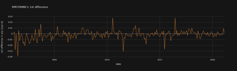
Upon quick graphical visualisation, it seems as though we ought to choose RMCPANNL's 1st difference
Checking For Stationarity Via Test Statistics
We can create a Python function for the three aforementioned test-statistics for stationarity: Augmented Dickey-Fuller (ADF), Phillips-Perron (PP) and the Kwiatkowski–Phillips–Schmidt–Shin (KPSS) ones.
For the ADF test, one may use the adfuller function from the statsmodels library (imported via the line from statsmodels.tsa.stattools import adfuller), but that library doesn't have functions for all the tests in question. the arch library does - however. So I will define a Python function Stationarity_Table returning all relevant arch stationarity results of interest:
import arch
from arch.unitroot import ADF, PhillipsPerron, KPSS
print(arch.__version__)
4.19
def Stationarity_Table(data = [df["RMCPANNL"]["yoy"].dropna(),
df["RMUNPTOTP"]["raw"].dropna()],
dataset_names = ["RMCPANNL", "RMUNPTOTP"],
tests = ["ADF", "PP", "KPSS"],
enumerate_data = False):
"""Stationarity_Table Version 1.0:
This function returns a Pandas data-frame with the results of the
Augmented Dickey-Fuller (ADF), Phillips-Perron (PP) and the
Kwiatkowski–Phillips–Schmidt–Shin (KPSS) stationarity tests from
the arch library.
Parameters:
----------
data: list
list of nan-less Pandas data-frames of number-series on which the test will be performed
Default: data = [df["RMCPANNL"]["yoy"].dropna(), df["RMUNPTOTP"]["raw"].dropna()]
dataset_names: list
List of strings of the names to show as columns in our resulted table
Default: dataset_names = ["RMCPANNL", "RMUNPTOTP"]
tests: list
List of strings of the stationarity tests wished.
You may choose between "ADF", "PP", and/or "KPSS".
Default: tests = ["ADF", "PP", "KPSS"]
Dependencies:
----------
pandas 1.2.3
numpy 1.19.5
arch 4.15 as ' from arch.unitroot import ADF, PhillipsPerron, KPSS '
Examples:
--------
>>> import DatastreamDSWS as dsws
>>> ds = dsws.Datastream(username = "insert dsws username here", password = "insert dsws password here")
>>>
>>> df_1 = ds.get_data(tickers = "RMCPANNL,RMUNPTOTP", # be carefulnot to put spaces in between elements here, or else these spaces will be included in column names.
>>> fields = "X", start = '2000-01-01', freq = 'M')
>>>
>>> Stationarity_Table(data = [df_1["RMCPANNL"]["X"].dropna(), df_1["RMUNPTOTP"]["X"].dropna()], dataset_names = ["RMCPANNL", "RMUNPTOTP"], tests = ["ADF", "PP", "KPSS"], enumerate_data = False)
"""
_columns, stationarity_test = [], []
for i in tests:
_columns.append((i, "Test-statistic", "")) # The ', ""' is there for the Pandas MultiIndex
_columns.append((i, "p-value", ""))
_columns.append((i, "Number of lags used", ""))
_columns.append(
(i,
"Number of observations used for the regression and critical values'calculation",
""))
_columns.append((i, "Critical values", '1%'))
_columns.append((i, "Critical values", '5%'))
_columns.append((i, "Critical values", '10%'))
_columns.append((i, "Null hypothesis", ""))
for d, _d in zip([D.astype(np.float64) for D in data], enumerate(data)):
if enumerate_data == True:
print(_d[0])
_tests, _data = [], []
if "ADF" in tests: _tests.append(ADF(d))
if "PP" in tests: _tests.append(PhillipsPerron(d))
if "KPSS" in tests: _tests.append(KPSS(d))
for i in _tests:
_data.append(i.stat)
_data.append(i.pvalue)
_data.append(i.lags)
_data.append(i.nobs)
for k in [i.critical_values[j] for j in i.critical_values]:
_data.append(k)
_data.append(i.null_hypothesis)
stationarity_test.append(
pd.DataFrame(
data = np.array(_data)[np.newaxis],
columns = pd.MultiIndex.from_tuples(_columns)).T)
stationarity_test_table = pd.concat(
stationarity_test, axis = 1, join = "inner")
stationarity_test_table = pd.DataFrame(
data = stationarity_test_table.values,
index = stationarity_test_table.index,
columns = dataset_names)
return stationarity_test_table
Stationarity_Table(
data = [df["RMCPANNL"]["yoy"].dropna(),
df["RMUNPTOTP"]["raw"].dropna(),
df["RMUNPTOTP"]["yoy"].dropna(),
df["RMXRUSD."]["raw"].dropna(),
df["RMXRUSD."]["yoy"].dropna(),
df["RMXREUR."]["raw"].dropna(),
df["RMXREUR."]["yoy"].dropna(),
df["RMGOVBALA"]["raw"].dropna(),
df["RMGOVBALA"]["yoy"].dropna(),
df["CLc1"]["Close Price 30D Moving Average"].dropna(),
df["CLc1"]["yoy"].dropna()],
dataset_names = ["RMCPANNL yoy",
"RMUNPTOTP raw","RMUNPTOTP yoy",
"RMXRUSD. raw", "RMXRUSD. yoy",
"RMXREUR. raw", "RMXREUR. yoy",
"RMGOVBALA raw", "RMGOVBALA yoy",
"CLc1 Close Price 30D Moving Average",
"CLc1 Close Price yoy"],
tests = ["ADF", "PP", "KPSS"],
enumerate_data = False)
# # for ' data ', one could use:
# [df[i][j].dropna() for i,j in zip(
# ["RMCPANNL", "RMUNPTOTP", "RMUNPTOTP",
# "RMXRUSD.", "RMXRUSD.", "RMXREUR.", "RMXREUR.",
# "RMGOVBALA", "RMGOVBALA", "CLc1", "CLc1"],
# ["yoy", "raw", "yoy", "raw", "yoy", "raw", "yoy",
# "raw", "yoy", "Close Price 30D Moving Average", "yoy"])]
| RMCPANNL yoy | RMUNPTOTP raw | RMUNPTOTP yoy | RMXRUSD. raw | RMXRUSD. yoy | RMXREUR. raw | RMXREUR. yoy | RMGOVBALA raw | RMGOVBALA yoy | CLc1 Close Price 30D Moving Average | CLc1 Close Price yoy | |||
| ADF | Test-statistic | -4.0516 | -2.2359 | -3.6895 | -1.5542 | -3.439 | -2.4889 | -2.642 | -0.0676 | -15.433 | -2.5897 | -2.9546 | |
| p-value | 0.00116 | 0.19348 | 0.00426 | 0.50657 | 0.0097 | 0.1182 | 0.08463 | 0.95257 | 2.93E-28 | 0.09515 | 0.03935 | ||
| Number of lags used | 15 | 15 | 15 | 1 | 13 | 1 | 14 | 15 | 0 | 2 | 13 | ||
| Number of observations used for the regression and critical values'calculation | 226 | 226 | 226 | 240 | 228 | 240 | 227 | 226 | 241 | 239 | 228 | ||
| Critical values | 1% | -3.4596 | -3.4596 | -3.4596 | -3.4579 | -3.4594 | -3.4579 | -3.4595 | -3.4596 | -3.4578 | -3.458 | -3.4594 | |
| 5% | -2.8744 | -2.8744 | -2.8744 | -2.8737 | -2.8743 | -2.8737 | -2.8744 | -2.8744 | -2.8736 | -2.8737 | -2.8743 | ||
| 10% | -2.5736 | -2.5736 | -2.5736 | -2.5732 | -2.5736 | -2.5732 | -2.5736 | -2.5736 | -2.5732 | -2.5733 | -2.5736 | ||
| Null hypothesis | The process contains a unit root. | The process contains a unit root. | The process contains a unit root. | The process contains a unit root. | The process contains a unit root. | The process contains a unit root. | The process contains a unit root. | The process contains a unit root. | The process contains a unit root. | The process contains a unit root. | The process contains a unit root. | ||
| PP | Test-statistic | -6.2226 | -2.6368 | -2.9359 | -1.4358 | -3.3385 | -2.4428 | -2.8822 | -6.6524 | -15.445 | -2.0948 | -3.1094 | |
| p-value | 5.18E-08 | 0.08563 | 0.04133 | 0.56501 | 0.01324 | 0.13002 | 0.04746 | 5.08E-09 | 2.84E-28 | 0.2466 | 0.02587 | ||
| Number of lags used | 15 | 15 | 15 | 15 | 15 | 15 | 15 | 15 | 15 | 15 | 15 | ||
| Number of observations used for the regression and critical values'calculation | 241 | 241 | 241 | 241 | 241 | 241 | 241 | 241 | 241 | 241 | 241 | ||
| Critical values | 1% | -3.4578 | -3.4578 | -3.4578 | -3.4578 | -3.4578 | -3.4578 | -3.4578 | -3.4578 | -3.4578 | -3.4578 | -3.4578 | |
| 5% | -2.8736 | -2.8736 | -2.8736 | -2.8736 | -2.8736 | -2.8736 | -2.8736 | -2.8736 | -2.8736 | -2.8736 | -2.8736 | ||
| 10% | -2.5732 | -2.5732 | -2.5732 | -2.5732 | -2.5732 | -2.5732 | -2.5732 | -2.5732 | -2.5732 | -2.5732 | -2.5732 | ||
| Null hypothesis | The process contains a unit root. | The process contains a unit root. | The process contains a unit root. | The process contains a unit root. | The process contains a unit root. | The process contains a unit root. | The process contains a unit root. | The process contains a unit root. | The process contains a unit root. | The process contains a unit root. | The process contains a unit root. |
Interpreting the stationarity table: As per the above, the null hypothesis of the ADF is that there is a unit root, with the alternative that there is no unit root. If the P-value is above a critical size, then we cannot reject that there is a unit root. If the process has a unit root, then it is a non-stationary time series. If the p-value is close to significant, then the critical values should be used to judge whether to reject the null.
Since ${ADF}_{{Test-statistic}_{RMCPANNL yoy}} \approx -6.025 < {ADF}_{{1\% Critical value}_{RMCPANNL yoy}} \approx -3.471$, we can reject the hypothesis that there is a unit root and presume our series to be stationary. Same conclusions can be taken from the PP and KPSS tests of our RMCPANNL data. This is an interesting finding since our graphical analysis suggested otherwise.
As aforementioned, differencing a time series $\{z\}_1^T$ once would render $\{z_2 - z_1, z_3 - z_2, ..., z_T - z_{T-1}\}$. Let's add the 1st difference of our data to our Pandas data-frame ```df```:
df["RMCPANNL", "yoy1d"] = df["RMCPANNL"]["yoy"].diff(1)
df["RMUNPTOTP", "yoy1d"] = df["RMUNPTOTP"]["yoy"].diff(1)
df["RMXRUSD.", "yoy1d"] = df["RMXRUSD."]["yoy"].diff(1)
df["RMXRUSD.", "yoy1d"] = df["RMXRUSD."]["yoy"].diff(1)
df["RMXREUR.", "yoy1d"] = df["RMXREUR."]["yoy"].diff(1)
df["RMGOVBALA", "yoy1d"] = df["RMGOVBALA"]["yoy"].diff(1)
df["CLc1", "yoy1d"] = df["CLc1"]["yoy"].diff(1)
df = df.sort_index(axis = 1)
df.dropna()
| Instrument | CLc1 | RMCPANNL | RMGOVBALA | RMUNPTOTP | RMXREUR. | RMXRUSD. | ||||||||||||
| Field | Close Price | Close Price 30D Moving Average | yoy | yoy1d | yoy | yoy1d | raw | yoy | yoy1d | raw | yoy | yoy1d | raw | yoy | yoy1d | raw | yoy | yoy1d |
| 15/02/2001 | 28.8 | 29.8113 | 0.07816 | -0.0217 | 0.4 | 0.001 | -601.2 | 0.30158 | -0.5786 | 1032.3 | -0.1373 | -0.0164 | 2.4729 | 0.34244 | 0.01994 | 2.68 | 0.43316 | 0.00924 |
| 15/03/2001 | 26.58 | 28.976 | -0.0423 | -0.1205 | 0.403 | 0.003 | -865.2 | 0.04746 | -0.2541 | 992.8 | -0.1491 | -0.0117 | 2.4849 | 0.34044 | -0.002 | 2.73 | 0.42188 | -0.0113 |
| 15/04/2001 | 28.2 | 27.25 | -0.0318 | 0.01048 | 0.375 | -0.028 | -1087.5 | -0.1019 | -0.1494 | 948.4 | -0.1675 | -0.0184 | 2.488 | 0.32956 | -0.0109 | 2.79 | 0.40909 | -0.0128 |
| 15/05/2001 | 28.98 | 27.9327 | 0.0575 | 0.08932 | 0.374 | -0.001 | -1404.5 | 0.02683 | 0.12874 | 890.8 | -0.1883 | -0.0208 | 2.491 | 0.34598 | 0.01642 | 2.85 | 0.39706 | -0.012 |
| 15/06/2001 | 28.53 | 28.6177 | -0.0403 | -0.0978 | 0.357 | -0.017 | -2268.9 | 0.25973 | 0.2329 | 840.3 | -0.2125 | -0.0242 | 2.4732 | 0.23846 | -0.1075 | 2.9 | 0.38095 | -0.0161 |
| ... | ... | ... | ... | ... | ... | ... | ... | ... | ... | ... | ... | ... | ... | ... | ... | ... | ... | ... |
| 15/10/2020 | 40.92 | 39.4793 | -0.2909 | -0.0379 | 0.0224 | -0.0021 | -76512 | 1.81579 | -0.0034 | 285.7 | 0.10437 | 0.00959 | 4.8733 | 0.02514 | -0.0004 | 4.14 | -0.0372 | 0.00465 |
| 15/11/2020 | 40.12 | 39.5773 | -0.2836 | 0.00733 | 0.0214 | -0.001 | -85982 | 1.47431 | -0.3415 | 290.7 | 0.12066 | 0.0163 | 4.8699 | 0.02131 | -0.0038 | 4.12 | -0.0441 | -0.0069 |
| 15/12/2020 | 47.59 | 43.203 | -0.2489 | 0.03465 | 0.0206 | -0.0008 | -105907 | 1.20275 | -0.2716 | 296.1 | 0.14812 | 0.02746 | 4.8707 | 0.01955 | -0.0018 | 4 | -0.0698 | -0.0257 |
| 15/01/2021 | 52.04 | 48.7013 | -0.1892 | 0.05969 | 0.0299 | 0.0093 | -112.3 | -0.8426 | -2.0454 | 292.2 | 0.12862 | -0.0195 | 4.8728 | 0.01973 | 0.00018 | 4 | -0.0719 | -0.0022 |
| 15/02/2021 | 59.73 | 53.606 | -0.0281 | 0.16113 | 0.0316 | 0.0017 | -8430.8 | -0.199 | 0.64362 | 293.5 | 0.14336 | 0.01474 | 4.8741 | 0.01909 | -0.0006 | 4.03 | -0.0799 | -0.008 |
241 rows × 18 columns
Stationarity_Table(
data = [
df[i]["yoy1d"].dropna()
for i in [
"RMCPANNL", "RMUNPTOTP", "RMXRUSD.",
"RMXREUR.", "RMGOVBALA", "CLc1"]],
dataset_names = [
"RMCPANNL yoy1d", "RMUNPTOTP yoy1d",
"RMXRUSD. yoy1d", "RMXREUR. yoy1d",
"RMGOVBALA yoy1d", "CLc1 Close Price yoy1d"],
tests = ["ADF", "PP"])
| RMCPANNL yoy1d | RMUNPTOTP yoy1d | RMXRUSD. yoy1d | RMXREUR. yoy1d | RMGOVBALA yoy1d | CLc1 Close Price yoy1d | |||
| ADF | Test-statistic | -3.9779 | -5.1251 | -5.8272 | -3.691 | -8.2178 | -8.5853 | |
| p-value | 0.00153 | 1.25E-05 | 4.05E-07 | 0.00424 | 6.55E-13 | 7.53E-14 | ||
| Number of lags used | 14 | 12 | 12 | 15 | 9 | 11 | ||
| Number of observations used for the regression and critical values'calculation | 226 | 228 | 228 | 225 | 231 | 229 | ||
| Critical values | 1% | -3.4596 | -3.4594 | -3.4594 | -3.4598 | -3.459 | -3.4592 | |
| 5% | -2.8744 | -2.8743 | -2.8743 | -2.8745 | -2.8741 | -2.8742 | ||
| 10% | -2.5736 | -2.5736 | -2.5736 | -2.5737 | -2.5735 | -2.5735 | ||
| Null hypothesis | The process contains a unit root. | The process contains a unit root. | The process contains a unit root. | The process contains a unit root. | The process contains a unit root. | The process contains a unit root. | ||
| PP | Test-statistic | -13.791 | -9.5569 | -9.553 | -10.36 | -57.826 | -7.7634 | |
| p-value | 8.94E-26 | 2.49E-16 | 2.54E-16 | 2.41E-18 | 0 | 9.33E-12 | ||
| Number of lags used | 15 | 15 | 15 | 15 | 15 | 15 | ||
| Number of observations used for the regression and critical values'calculation | 240 | 240 | 240 | 240 | 240 | 240 | ||
| Critical values | 1% | -3.4579 | -3.4579 | -3.4579 | -3.4579 | -3.4579 | -3.4579 | |
| 5% | -2.8737 | -2.8737 | -2.8737 | -2.8737 | -2.8737 | -2.8737 | ||
| 10% | -2.5732 | -2.5732 | -2.5732 | -2.5732 | -2.5732 | -2.5732 | ||
| Null hypothesis | The process contains a unit root. | The process contains a unit root. | The process contains a unit root. | The process contains a unit root. | The process contains a unit root. | The process contains a unit root. |
Now they're all stationary. We ought to use datasets treated similarly for consistency (e.g.: compare 'RMCPANNL yoy1d' with 'RMUNPTOTP yoy1d' rather than with 'RMUNPTOTP yoy'), so we will use the ones shown in the last table (i.e.: 'yoy1d' datasets).
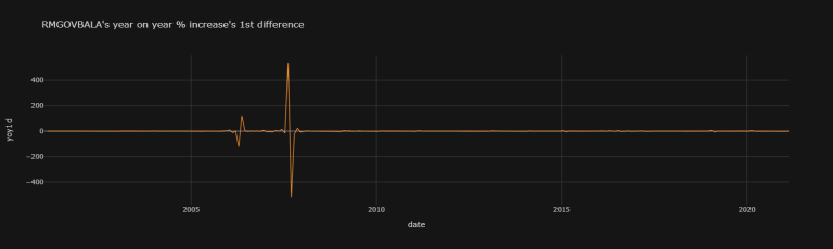
N.B.: The RMGOVBALA yoy1d dataset is causing issues with the KPSS test, but that one is only for weak stationarity, and is not of as much interest to us in our study - I just wanted to include it to portray the extent of the Stationarity_Table function. The RMGOVBALA yoy1d dataset is causing issues with the KPSS test because of its large variance, as can be seen in this graph:
df["RMGOVBALA"]["yoy1d"].iplot(
theme = "solar", xTitle = "date", yTitle = "yoy1d",
title = "RMGOVBALA's year on year % increase's 1st difference")
Modelling
Now we will look at which ARMA-family model to implement. We'll look at the best model orders to choose before (ex-ante) and after (ex-post) going through modelling procedures.
Ex-Ante Parameter Identification: Autocorrelation and Partial Autocorrelation Functions
To figure out our parameter identification (i.e.: what lags to use in our model), we may want to plot ACF and PACF diagrams:
import matplotlib.pyplot as plt
import statsmodels.api as sm
N.B.: the semicolon at the end of the code for our plots below is there to avoid duplicates.
sm.graphics.tsa.plot_acf(x = df["RMCPANNL"]["yoy1d"].dropna(), lags = 25);
sm.graphics.tsa.plot_pacf(x = df["RMCPANNL"]["yoy1d"].dropna(), lags = 25);
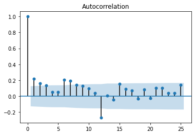
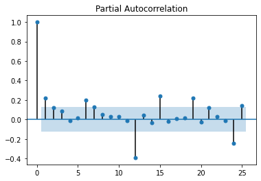
From these graphs (also known as (a.k.a.): correlograms), we could identify an AR(1,4,5) (non-consecutive) model; but the MA part is harder to decipher. Let's have a look at how those models would fair:
- 1st: a simple ARMA(5,2) model (i.e.: a SARIMA(5,0,2) model), then
- 2nd: a SARIMA(5,0,2)(1, 0, 0)12 model:
ARMA(5,2)
from statsmodels.tsa.arima.model import ARIMA
arima502c = ARIMA(endog = np.array(df["RMCPANNL"]["yoy1d"].dropna()),
order = (5, 0, 2), # We don't need to difference our data again, so 'd' is set to 0.
trend = "c")
arima502c_fit = arima502c.fit()
arima502c_fit.summary()
| SARIMAX Results | ||||||
| Dep. Variable: | y | No. Observations: | 241 | |||
| Model: | ARIMA(5, 0, 2) | Log Likelihood | 847.684 | |||
| Date: | Mon, 19 Apr 2021 | AIC | -1677.4 | |||
| Time: | 14:33:02 | BIC | -1646 | |||
| Sample: | 0 | HQIC | -1664.7 | |||
| -241 | ||||||
| Covariance Type: | opg | |||||
| coef | std err | z | P>|z| | [0.025 | 0.975] | |
| const | -0.0015 | 0.001 | -1.913 | 0.056 | -0.003 | 3.66E-05 |
| ar.L1 | 0.0858 | 17.28 | 0.005 | 0.996 | -33.783 | 33.955 |
| ar.L2 | 0.0603 | 8.153 | 0.007 | 0.994 | -15.919 | 16.039 |
| ar.L3 | 0.1161 | 1.11 | 0.105 | 0.917 | -2.059 | 2.292 |
| ar.L4 | -0.0028 | 1.219 | -0.002 | 0.998 | -2.393 | 2.387 |
| ar.L5 | -0.0027 | 0.782 | -0.003 | 0.997 | -1.535 | 1.53 |
| ma.L1 | 0.0995 | 17.281 | 0.006 | 0.995 | -33.77 | 33.969 |
| ma.L2 | 0.0615 | 5.295 | 0.012 | 0.991 | -10.317 | 10.44 |
| sigma2 | 5.15E-05 | 3.30E-06 | 15.595 | 0 | 4.51E-05 | 5.80E-05 |
| Ljung-Box (L1) (Q): | 0 | Jarque-Bera (JB): | 274.28 | |||
| Prob(Q): | 0.96 | Prob(JB): | 0 | |||
| Heteroskedasticity (H): | 0.53 | Skew: | -0.6 | |||
| Prob(H) (two-sided): | 0.01 | Kurtosis: | 8.09 | |||
Warnings:
[1] Covariance matrix calculated using the outer product of gradients (complex-step).
SARIMA(5,0,2)(1, 0, 0)12
s1arima502c = ARIMA(endog = np.array(df["RMCPANNL"]["yoy1d"].dropna()),
order = (5, 0, 2),
trend = "c",
seasonal_order = (1, 0, 0, 12))
s1arima502c_fit = s1arima502c.fit()
s1arima502c_fit.summary()
| SARIMAX Results | ||||||
| Dep. Variable: | y | No. Observations: | 241 | |||
| Model: | ARIMA(5, 0, 2)x(1, 0, [], 12) | Log Likelihood | 868.387 | |||
| Date: | Mon, 19 Apr 2021 | AIC | -1716.8 | |||
| Time: | 14:33:04 | BIC | -1681.9 | |||
| Sample: | 0 | HQIC | -1702.7 | |||
| -241 | ||||||
| Covariance Type: | opg | |||||
| coef | std err | z | P>|z| | [0.025 | 0.975] | |
| const | -0.0015 | 0.001 | -1.856 | 0.063 | -0.003 | 8.27E-05 |
| ar.L1 | 0.0761 | 2.209 | 0.034 | 0.973 | -4.253 | 4.405 |
| ar.L2 | 0.0641 | 1.92 | 0.033 | 0.973 | -3.698 | 3.827 |
| ar.L3 | 0.2522 | 0.31 | 0.815 | 0.415 | -0.355 | 0.859 |
| ar.L4 | 0.052 | 0.474 | 0.11 | 0.913 | -0.877 | 0.981 |
| ar.L5 | 0.0496 | 0.366 | 0.136 | 0.892 | -0.667 | 0.766 |
| ma.L1 | 0.1203 | 2.203 | 0.055 | 0.956 | -4.198 | 4.439 |
| ma.L2 | 0.0607 | 1.679 | 0.036 | 0.971 | -3.231 | 3.352 |
| ar.S.L12 | -0.4396 | 0.042 | -10.401 | 0 | -0.522 | -0.357 |
| sigma2 | 4.29E-05 | 2.85E-06 | 15.025 | 0 | 3.73E-05 | 4.85E-05 |
| Ljung-Box (L1) (Q): | 0.01 | Jarque-Bera (JB): | 142.78 | |||
| Prob(Q): | 0.92 | Prob(JB): | 0 | |||
| Heteroskedasticity (H): | 0.53 | Skew: | -0.56 | |||
| Prob(H) (two-sided): | 0 | Kurtosis: | 6.6 | |||
Warnings:
[1] Covariance matrix calculated using the outer product of gradients (complex-step).
Ex-Post Parameter Identification: Information Criteria and Mean of Absolute & squared Errors
Graphical Analysis
After having fit a model, one may try to look at the residuals to compare models:
models_resid = pd.DataFrame(
data = {'arima502c residuals' : arima502c_fit.resid,
's1arima502c residuals' : s1arima502c_fit.resid})
models_resid.iplot(
theme = "solar", xTitle = "date",
yTitle = "residuals (%)",
title = "arima502c and s1arima502c models' residuals")
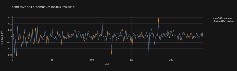
Looking at such graphical information is not simple. (i) Not only is it arbitrary to chose a model over another from graphical information (ii) it quickly becomes difficult when comparing many models together. That's why we may compare them instead with performance measurements such as Information Criteria:
Information Criteria
def IC_Table(models_fit, models_name):
return pd.DataFrame(
data = [[i.aic, i.aicc, i.bic, i.hqic]
for i in models_fit],
columns = ['AIC', 'AICC', 'BIC', 'HQIC'],
index = [str(i) for i in models_name])
# ' ic ' standing for 'information criteria':
ic0 = IC_Table(models_fit = [arima502c_fit, s1arima502c_fit],
models_name = ['arima502c', 's1arima502c'])
ic0
| AIC | AICC | BIC | HQIC | |
| arima502c | -1677.4 | -1676.6 | -1646 | -1664.7 |
| s1arima502c | -1716.8 | -1715.8 | -1681.9 | -1702.7 |
We can similarly go through each permutation within limits of our SARIMA model's parameters, and go beyond just recording IC information - including mean squared error (MSE) and sum of squared error (SSE, a.k.a.: RSS) information too.
Mean Squared Errors and Sum of squared Errors
We can define the below function to return a table of
- the Akaike information criterion (AIC),
- the AICc (AIC with a correction for small sample sizes),
- the Bayesian information criterion (BIC) (aka Schwarz criterion (also SBC, SBIC)) and
- the Hannan-Quinn information criterion (HQC) as well as
- the Mean Squared Errors (MSE) and
- the Sum of Squared Errors (SSE) (aka: residual sum of squares (RSS))
of any specified ARIMAX model, and then choose the one providing the lowest (of any one chosen error measure above) as the optimal model of choice:
import itertools # We need this library to iteratethrough each permutation of exogenous variable possible
N.B.: Note that we need to lag our exogenous variables since we are putting ourselves in the shoes of a programmer who is using past values to predict tomorrow's.
def Reg_Perm_Table(endog = np.array(df.dropna()["RMCPANNL"]["yoy1d"][1:].values.tolist()), # the ' [1:] ' is here to get same number of figures as in our exogenous variables.
exogenous = [df.dropna()[i]["yoy1d"].shift(1)[1:].values.tolist() # ' .shift(1) ' is here to get lagged values; the ' [1:] ' is there to remove the 0th value which is nan due to the lagging.
for i in ["CLc1", "RMGOVBALA", "RMUNPTOTP", "RMXREUR.", "RMXRUSD."]],
exogenous_names = ["CLc1", "RMGOVBALA", "RMUNPTOTP", "RMXREUR.", "RMXRUSD."],
d = [0], D = [0], s = [12],
p = range(5), q = range(5),
P = range(5), Q = range(5),
trend = "c",
print_progress = False,
try_loop = False,
save_model_fit = False,
lowest_no = 3):
""" Reg_Perm_Table Version 1.0:
This Python function ' Reg_Perm_Table ' goes through each permutation of possible ARIMA orders
(chosen in parameters d, D, s, p, P, q, and Q) and exogenous variables and returns two Pandas
data-frames (table and lowest) to help decide (i) the optimal exogenous variables to use,
(ii) the optimal order of our ARIMA model to use.
' table ' consists of the Akaike information criterion (AIC),
the AICc (AIC with a correction for small sample sizes),
the Bayesian information criterion (BIC) (aka Schwarz criterion (also SBC, SBIC)) and
the Hannan-Quinn information criterion (HQC)
as well as the Mean Squared Errors (MSE) and
the Sum of Squared Errors (SSE) (aka: residual sum of squares (RSS)) of any specified ARIMAX model.
' lowest ' consists of the name of all models with lowest values of all the metrics in ' table '.
For more information on ARIMA orders (both (i) orders p, d, and q and (ii) seasonal orders P, D,
Q and s), look at the statsmodels website:
https://www.statsmodels.org/stable/generated/statsmodels.tsa.arima.model.ARIMA.html
Parameters:
----------
endog: Numpy array
Numpy array of a list of values used as endogenous variables in our ARIMAX model.
Defaulted to: np.array(df.dropna()["RMCPANNL"]["yoy1d"][1:].values.tolist()) # The ' [1:] ' is here to get same number of figures as in our exogenous variables.
exogenous: list
List of lists of each of the exogenous variables wished. can be set to ' None ' BUT
IT CANNOT CONSIST OF ONLY ONE ELEMENT.
Defaulted to: exogenous = [df.dropna()[i]["yoy1d"].shift(1)[1:].values.tolist() for i in ["CLc1", "RMGOVBALA", "RMUNPTOTP", "RMXREUR.", "RMXRUSD."]] # ' .shift(1) ' is here to get lagged values; the ' [1:] ' is there to remove the 0th value which is nan due to the lagging.
exogenous_names: list
list of strings of the names of the exogenous variables wished to be seen in
the outputed data-frames. They have to be in the same order as in the ' exogenous ' variables.
Defaulted to: exogenous_names = ["CLc1", "RMGOVBALA", "RMUNPTOTP", "RMXREUR.", "RMXRUSD."]
p: list
list of the ARIMA order 'p' that the user wishes to iteratethrough. This can be a range.
Defaulted to: p = [0]
d: list
list of the ARIMA order 'd' that the user wishes to iteratethrough. This can be a range.
Defaulted to: d = [0]
q: list
list of the ARIMA order 'q' that the user wishes to iteratethrough. This can be a range.
Defaulted to: q = [0]
P: list
list of the ARIMA seasonal order 'P' that the user wishes to iteratethrough. This can be a range.
Defaulted to: P = [0]
D: list
list of the ARIMA seasonal order 'D' that the user wishes to iteratethrough. This can be a range.
Defaulted to: D = [0]
Q: list
list of the ARIMA seasonal order 'Q' that the user wishes to iteratethrough. This can be a range.
Defaulted to: Q = [0]
s: list
list of the ARIMA seasonal order 's' that the user wishes to iteratethrough. This can be a range.
Defaulted to: s = [0]
trend: str
str{‘n’,’c’,’t’,’ct’} or 'iterate-able', optional as per statsmodels.tsa.arima.model.ARIMA.
Defaulted to: trend = "c"
print_progress: Boolean
If True, then a summary of each fitted model will appear in order of execution.
Defaulted to: print_progress = False
try_loop: Boolean
If true, a try and except (then pass) loop is used over the model specification and
fitting. If that part of the code fails, it will just ignore the model that caused an error from the output.
Defaulted to: try_loop = False
save_model_fit: Boolean
ARIMA model fit's Python objects take up a lot of memory, so they are not saved. If
this argument is st to True, our function then returns a new list full of each fit objects in the order they
were executed called ' model_fit_list '; the function returns: table, model_fit_list, lowest
Defaulted to: save_model_fit = False
lowest_no: int
the returned table ' lowest ' provides the name of each model with lowest AIC, AICC, BIC,
HQIC, MSE and SSE up to the 3rd lowest value by default, but you can change that here.
Defaulted to: lowest_no = 3
Dependencies:
----------
itertools
numpy as np: version 1.19.5
pandas as pd: version 1.2.3
from statsmodels.tsa.arima.model import ARIMA: version 0.11.1
Examples:
--------
>>> import DatastreamDSWS as dsws # Using LSEG Refinitiv's Datastream Python API named DataStreem Web Service (DSWS).
>>> ds = dsws.Datastream(username = "insert dsws username here", password = "insert dsws password here")
>>>
>>> df_1 = ds.get_data(tickers = "RMCPANNL,RMGOVBALA,RMXRUSD.", # be carefulnot to put spaces in between elements here, or else these spaces will be included in column names.
>>> fields = "X", start = '2000-01-01', freq = 'M')
>>>
>>> Reg_Perm_Table(endog = np.array(df_1.dropna()["RMCPANNL"]["X"][1:].values.tolist()), # the ' [1:] ' is here to get same number of figures as in our exogenous variables.
>>> exogenous = [df_1.dropna()[i]["X"].shift(1)[1:].values.tolist() # ' .shift(1) ' is here to get lagged values; the ' [1:] ' is there to remove the 0th value which is nan due to the lagging.
>>> for i in ["RMXRUSD.", "RMGOVBALA"]],
>>> exogenous_names = ["RMXRUSD.", "RMGOVBALA"])
"""
model_table_data, model_fit_list, models_name_list = [], [], [] # Lists to be appended.
for _p in p: # Going through each permutation of possible arguments.
for _d in d:
for _q in q:
for _P in P:
for _D in D:
for _Q in Q:
for _s in s:
def Modelling(exog1, endog1 = endog,
order1 = (_p, _d, _q), trend1 = trend,
seasonal_order1 = (_P, _D, _Q, _s)):
# global?
return ARIMA(endog = endog1, exog = exog1,
order = order1, trend = trend1,
seasonal_order = (_P, _D, _Q, _s)).fit()
if exogenous != None:
for j in range(1,len(exogenous_names)+1):
for i,i_name in zip(itertools.combinations(exogenous, r = j),
itertools.combinations(exogenous_names, r = j)):
if try_loop == True:
try: # statsmodels' ARIMA function does not work 100% of the time.
model = Modelling(exog1 = np.array(i).T)
model_table_data.append(
[model.aic, model.aicc, model.bic,
model.hqic, model.mse, model.sse])
if save_model_fit == True: model_fit_list.append(model)
models_name_list.append(
f"sarima{_p},{_d},{_q},{_P},{_D},{_Q},{_s},{trend},exo={i_name}")
if print_progress == True: # For debugging.
print(models_name_list[-1])
display(model_fit_list[-1].summary())
except:
pass
else: # i.e.: if try_loop != True
model = Modelling(exog1 = np.array(i).T)
model_table_data.append(
[model.aic, model.aicc, model.bic,
model.hqic, model.mse, model.sse])
if save_model_fit == True: model_fit_list.append(model)
models_name_list.append(
f"sarima{_p},{_d},{_q},{_P},{_D},{_Q},{_s},{trend},exo={i_name}")
if print_progress == True: # For debugging.
print(models_name_list[-1])
display(model_fit_list[-1].summary())
elif exogenous == None:
if try_loop == True:
try: # statsmodels' ARIMA function does not work 100% of the time.
model = Modelling(exog1 = None)
model_table_data.append(
[model.aic, model.aicc, model.bic,
model.hqic, model.mse, model.sse])
if save_model_fit == True: model_fit_list.append(model)
models_name_list.append(
f"sarima{_p},{_d},{_q},{_P},{_D},{_Q},{_s},{trend},exo={i_name}")
if print_progress == True: # For debugging.
print(models_name_list[-1])
display(model_fit_list[-1].summary())
except:
pass
else: # i.e.: if try_loop != True
model = Modelling(exog1 = None)
model_table_data.append(
[model.aic, model.aicc, model.bic,
model.hqic, model.mse, model.sse])
if save_model_fit == True: model_fit_list.append(model)
models_name_list.append(
f"sarima{_p},{_d},{_q},{_P},{_D},{_Q},{_s},{trend},exo={i_name}")
if print_progress == True: # For debugging.
print(models_name_list[-1])
display(model_fit_list[-1].summary())
table = pd.DataFrame(
data = model_table_data,
columns = ['AIC', 'AICC', 'BIC', 'HQIC', "MSE", "SSE"],
index = [str(i) for i in models_name_list]) # Just like the previously defined 'IC_Table' function.
if lowest_no == None or lowest_no == False:
if save_model_fit == True:
return table, model_fit_list
else:
return table
else:
if lowest_no == 1:
lowest_index = ["1st lowest"]
elif lowest_no == 2:
lowest_index = [f"{i} lowest" for i in ['1st', '2nd']]
elif lowest_no == 3:
lowest_index = [f"{i} lowest" for i in ['1st', '2nd', '3rd']]
elif lowest_no > 3:
lowest_index = [f"{i} lowest"
for i in list(['1st', '2nd', '3rd'] +
[f"{j}th" for j in range(4, lowest_no + 1)])]
else:
print(f"{lowest_no} should be a positive integer")
lowest = pd.DataFrame({'AIC': table.nsmallest(lowest_no, 'AIC').index,
'AICC': table.nsmallest(lowest_no, 'AICC').index,
'BIC': table.nsmallest(lowest_no, 'BIC').index,
'HQIC': table.nsmallest(lowest_no, 'HQIC').index,
'MSE': table.nsmallest(lowest_no, 'MSE').index,
'SSE': table.nsmallest(lowest_no, 'SSE').index},
index = lowest_index)
if save_model_fit == True:
return table, model_fit_list, lowest
else:
return table, lowest
Now let's put this Python function into practice:
# We get a lot of 'Maximum Likelihood optimization failed to converge.
# Check mle_retvals' error messages, this cell will remove them.
# You don't need to remove them, it's just neater to.
import warnings
from statsmodels.tools.sm_exceptions import ConvergenceWarning
warnings.simplefilter('ignore', ConvergenceWarning)
# This step takes a long while
test1_df, test1_lowest = Reg_Perm_Table(p = [1])
Let's have a look at that table returned:
| AIC | AICC | BIC | HQIC | MSE | SSE | |
| sarima1,0,0,0,0,0,12,c,exo=('CLc1',) | -1067.6 | -1067.4 | -1055.4 | -1062.7 | 6.8E-05 | 0.01073 |
| sarima1,0,0,0,0,0,12,c,exo=('RMGOVBALA',) | -1067 | -1066.7 | -1054.7 | -1062 | 6.8E-05 | 0.01078 |
| sarima1,0,0,0,0,0,12,c,exo=('RMUNPTOTP',) | -1067.7 | -1067.4 | -1055.4 | -1062.7 | 6.7E-05 | 0.01073 |
| sarima1,0,0,0,0,0,12,c,exo=('RMXREUR.',) | -1067 | -1066.8 | -1054.8 | -1062 | 6.8E-05 | 0.01078 |
| sarima1,0,0,0,0,0,12,c,exo=('RMXRUSD.',) | -1069.2 | -1068.9 | -1056.9 | -1064.2 | 6.7E-05 | 0.01063 |
| ... | ... | ... | ... | ... | ... | ... |
| sarima1,0,4,4,0,4,12,c,exo=('CLc1', 'RMGOVBALA', 'RMUNPTOTP', 'RMXRUSD.') | -1047.2 | -1041.8 | -988.92 | -1023.6 | 6.3E-05 | 0.01005 |
| sarima1,0,4,4,0,4,12,c,exo=('CLc1', 'RMGOVBALA', 'RMXREUR.', 'RMXRUSD.') | -1047.9 | -1042.4 | -989.59 | -1024.2 | 6.3E-05 | 0.01002 |
| sarima1,0,4,4,0,4,12,c,exo=('CLc1', 'RMUNPTOTP', 'RMXREUR.', 'RMXRUSD.') | -1057.4 | -1051.9 | -999.09 | -1033.7 | 0.00006 | 0.00951 |
| sarima1,0,4,4,0,4,12,c,exo=('RMGOVBALA', 'RMUNPTOTP', 'RMXREUR.', 'RMXRUSD.') | -1043.1 | -1037.6 | -984.75 | -1019.4 | 6.5E-05 | 0.01029 |
| sarima1,0,4,4,0,4,12,c,exo=('CLc1', 'RMGOVBALA', 'RMUNPTOTP', 'RMXREUR.', 'RMXRUSD.') | -1048.2 | -1042.1 | -986.82 | -1023.3 | 6.2E-05 | 0.00994 |
3875 rows × 6 columns
Let's have a look at that table lowest returned:
test1_lowest
| AIC | AICC | BIC | HQIC | MSE | SSE | |
| 1st lowest | sarima1,0,1,0,0,0,12,c,exo=('RMUNPTOTP', 'RMXR... | sarima1,0,1,0,0,0,12,c,exo=('RMUNPTOTP', 'RMXR... | sarima1,0,0,0,0,0,12,c,exo=('RMXRUSD.',) | sarima1,0,1,0,0,0,12,c,exo=('RMUNPTOTP',) | sarima1,0,4,4,0,0,12,c,exo=('RMUNPTOTP', 'RMXR... | sarima1,0,4,4,0,0,12,c,exo=('RMUNPTOTP', 'RMXR... |
| 2nd lowest | sarima1,0,4,0,0,2,12,c,exo=('RMUNPTOTP', 'RMXR... | sarima1,0,1,0,0,0,12,c,exo=('RMUNPTOTP',) | sarima1,0,1,0,0,0,12,c,exo=('RMUNPTOTP',) | sarima1,0,1,0,0,0,12,c,exo=('RMXRUSD.',) | sarima1,0,4,4,0,0,12,c,exo=('CLc1', 'RMUNPTOTP... | sarima1,0,4,4,0,0,12,c,exo=('CLc1', 'RMUNPTOTP... |
| 3rd lowest | sarima1,0,4,0,0,0,12,c,exo=('RMUNPTOTP', 'RMXR... | sarima1,0,4,0,0,0,12,c,exo=('RMUNPTOTP',) | sarima1,0,1,0,0,0,12,c,exo=('RMXRUSD.',) | sarima1,0,1,0,0,0,12,c,exo=('CLc1',) | sarima1,0,4,4,0,3,12,c,exo=('CLc1', 'RMUNPTOTP... | sarima1,0,4,4,0,3,12,c,exo=('CLc1', 'RMUNPTOTP... |
Pickle
It is quite time consuming to request DSWS for all these codes. Furthermore, the table test1_df is rather large, and we only accounted for p, q, P, Q values up to (but not including) 3. What we could do is save our table in a file outside our code, then delete our table in our code, continue our analysis with test2_df and compare the two afterwards. Let's save our progress this far using Pickle. Since this is a step that can overwrite existing files, I commented them out. Feel free to uncomment them back in if you would like to save your data:
# need to ' pip install pickle-mixin '
import pickle
# To save data out:
pickle_out = open("Regression_Permutation_Table1.pickle","wb") # This creates the '.pickle' file where our data of choice will be saved. ' wb ' stand for 'write bytes'.
pickle.dump((test1_df, test1_lowest), # ' (test1_df, test1_lowest) ' are the two data-frames we choose to save.
pickle_out) # ' pickle_out ' specifies the '.pickle' file in which we want to write (actually: overwrite - everything previously in that file will be overwritten)
pickle_out.close() # We need to close this '.pickle' file; leaving it open could corrupt it.
# # To load data in:
# pickle_in = open("Regression_Permutation_Table2.pickle","rb") # ' rb ' stand for 'read bytes'.
# test1_df, test1_lowest = pickle.load(pickle_in)
# pickle_in.close() # We ought to close the file we opened to allow any other programs access if they need it.
As aforementioned, let's delete our tables in our code for now - after having saved them outside our code:
del test1_df
del test1_lowest
Now let's continue with our examination:
test2_df, test2_lowest = Reg_Perm_Table(p = [2])
pickle_out = open("Regression_Permutation_Table2.pickle","wb")
pickle.dump((test2_df, test2_lowest), pickle_out)
pickle_out.close()
del test2_df
test3_df, test3_lowest = Reg_Perm_Table(p = [3])
pickle_out = open("Regression_Permutation_Table3.pickle","wb")
pickle.dump((test3_df, test3_lowest), pickle_out)
pickle_out.close()
del test3_df
test4_df, test4_lowest = Reg_Perm_Table(p = [4], try_loop = True) # We tripped on some problems with this one, so used the ' try_loop '.
pickle_out = open("Regression_Permutation_Table4.pickle","wb")
pickle.dump((test4_df, test4_lowest), pickle_out)
pickle_out.close()
del test4_df
test5_df, test5_lowest = Reg_Perm_Table(p = [5])
pickle_out = open("Regression_Permutation_Table5.pickle","wb")
pickle.dump((test5_df, test5_lowest), pickle_out)
pickle_out.close()
del test5_df
pmdarima
If we knew which exogenous variables to use, we could have used pmdarima to find the best model specification too:
import pmdarima # Install via ' pip install pmdarima '
pmdarima.arima.auto_arima(
y = np.array(df.dropna()["RMCPANNL"]["yoy1d"][1:]),
X = None,
d = 1, # The order of first-differencing. If None (by default), the value will automatically be selected based on the results of the test (i.e., either the Kwiatkowski–Phillips–Schmidt–Shin, Augmented Dickey-Fuller or the Phillips–Perron test will be conducted to find the most probable value). Must be a positive integer or None. Note that if d is None, the runtime could be significantly longer.
start_p = 0, max_p = 7,
start_q = 0, max_q = 7,
D = None, max_D = 1,
start_P = 0, max_P = 2,
start_Q = 0, max_Q = 2,
m = 12, # The period for seasonal differencing, m refers to the number of periods in each season. For example, m is 4 for quarterly data, 12 for monthly data, or 1 for annual (non-seasonal) data. Default is 1. Note that if m == 1 (i.e., is non-seasonal), seasonal will be set to False. For more information on setting this parameter, see Setting m.
seasonal = True,
stationary = False,
information_criterion = 'aic',
test = 'kpss', # Type of unit root test to use in order to detect stationarity if stationary is False and d is None. Default is ‘kpss’ (Kwiatkowski–Phillips–Schmidt–Shin).
seasonal_test = 'ocsb', # This determines which seasonal unit root test is used if seasonal is True and D is None. Default is ‘OCSB’.
stepwise = True, # Whether to use the stepwise algorithm outlined in Hyndman and Khandakar (2008) to identify the optimal model parameters. The stepwise algorithm can be significantly faster than fitting all (or a random subset of) hyper-parameter combinations and is less likely to over-fit the model.
method = 'lbfgs', # The method determines which solver from scipy.optimize is used
maxiter = 40)
ARIMA(maxiter=40, order=(0, 1, 1), scoring_args={},
seasonal_order=(0, 0, 1, 12), suppress_warnings=True)
Unfortunately, we don't know what permutation of exogenous variables is best, and Information-Criteria-optimisation methods are thus not sufficient.
Optimal model
Finally, let's compare our two tables to check the lowest MSE and SSE:
# To load data in:
for j in range(1,6):
exec(f"pickle_in = open('Regression_Permutation_Table{j}.pickle','rb')") # ' rb ' stand for 'read bytes'.
exec(f"test{j}_df, test{j}_lowest = pickle.load(pickle_in)")
exec(f"pickle_in.close()") # We ought to close the file we opened to allow any other programs access if they need it.
for j in range(1,6):
# ' list(set( ' is there to return unique elements in case the same model has both the lowest MSE and SSE
# if you think about it, they should always be the same.
exec(f"display(test{j}_df.loc[list(set([i for i in test{j}_lowest[['MSE', 'SSE']].loc['1st lowest']]))])")
| AIC | AICC | BIC | HQIC | MSE | SSE | |
| sarima1,0,4,4,0,0,12,c,exo=('RMUNPTOTP', 'RMXRUSD.') | -1070.6 | -1068.1 | -1030.7 | -1054.4 | 5.9E-05 | 0.00946 |
| AIC | AICC | BIC | HQIC | MSE | SSE | |
| sarima2,0,4,1,0,4,12,c,exo=('CLc1', 'RMUNPTOTP', 'RMXRUSD.') | -1064.8 | -1060.9 | -1015.7 | -1044.8 | 5.9E-05 | 0.00944 |
| AIC | AICC | BIC | HQIC | MSE | SSE | |
| sarima3,0,4,4,0,0,12,c,exo=('CLc1', 'RMUNPTOTP', 'RMXRUSD.') | -1073.9 | -1070.1 | -1024.8 | -1054 | 5.6E-05 | 0.00896 |
| AIC | AICC | BIC | HQIC | MSE | SSE | |
| sarima4,0,4,4,0,0,12,c,exo=('CLc1', 'RMUNPTOTP', 'RMXRUSD.') | -1070 | -1065.7 | -1017.8 | -1048.8 | 5.7E-05 | 0.00904 |
| AIC | AICC | BIC | HQIC | MSE | SSE | |
| sarima5,0,4,4,0,0,12,c,exo=('RMUNPTOTP', 'RMXRUSD.') | -1072.2 | -1067.9 | -1020.1 | -1051.1 | 5.6E-05 | 0.00892 |
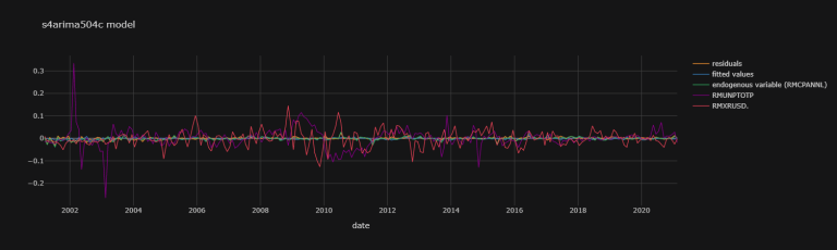
Thus, the best model out of our choices is the 'sarima5,0,4,4,0,0,12,c,exo=('RMUNPTOTP', 'RMXRUSD.')' model (best as in SSE and MSE reducing):
s4arima504c = ARIMA(endog = np.array(df.dropna()["RMCPANNL"]["yoy1d"][1:].values.tolist()),
exog = np.array([df.dropna()[i]["yoy1d"].shift(1)[1:].values.tolist()
for i in ["RMUNPTOTP", "RMXRUSD."]]).T,
order = (5, 0, 4),
trend = "c",
seasonal_order = (4, 0, 0, 12))
s4arima504c_fit = s4arima504c.fit()
s4arima504c_fit.summary()
| SARIMAX Results | ||||||
| Dep. Variable: | y | No. Observations: | 240 | |||
| Model: | ARIMA(5, 0, 4)x(4, 0, [], 12) | Log Likelihood | 892.165 | |||
| Date: | Mon, 19 Apr 2021 | AIC | -1750.3 | |||
| Time: | 14:33:44 | BIC | -1691.2 | |||
| Sample: | 0 | HQIC | -1726.5 | |||
| -240 | ||||||
| Covariance Type: | opg | |||||
| coef | std err | z | P>|z| | [0.025 | 0.975] | |
| const | -0.0013 | 0.001 | -1.947 | 0.052 | -0.003 | 8.87E-06 |
| x1 | -0.0066 | 0.014 | -0.484 | 0.629 | -0.033 | 0.02 |
| x2 | 0.0167 | 0.014 | 1.188 | 0.235 | -0.011 | 0.044 |
| ar.L1 | 0.4023 | 0.445 | 0.905 | 0.366 | -0.469 | 1.274 |
| ar.L2 | 0.264 | 0.596 | 0.443 | 0.658 | -0.904 | 1.432 |
| ar.L3 | 0.1468 | 0.31 | 0.473 | 0.636 | -0.461 | 0.755 |
| ar.L4 | -0.1802 | 0.435 | -0.415 | 0.678 | -1.032 | 0.672 |
| ar.L5 | 0.2342 | 0.103 | 2.266 | 0.023 | 0.032 | 0.437 |
| ma.L1 | -0.2364 | 0.446 | -0.53 | 0.596 | -1.11 | 0.637 |
| ma.L2 | -0.2758 | 0.555 | -0.497 | 0.619 | -1.363 | 0.812 |
| ma.L3 | -0.0235 | 0.327 | -0.072 | 0.943 | -0.664 | 0.617 |
| ma.L4 | 0.1263 | 0.429 | 0.294 | 0.768 | -0.714 | 0.967 |
| ar.S.L12 | -0.8138 | 0.08 | -10.118 | 0 | -0.971 | -0.656 |
| ar.S.L24 | -0.6277 | 0.101 | -6.204 | 0 | -0.826 | -0.429 |
| ar.S.L36 | -0.3844 | 0.103 | -3.746 | 0 | -0.586 | -0.183 |
| ar.S.L48 | -0.1285 | 0.085 | -1.517 | 0.129 | -0.295 | 0.038 |
| sigma2 | 3.25E-05 | 2.55E-06 | 12.775 | 0 | 2.75E-05 | 3.75E-05 |
| Ljung-Box (L1) (Q): | 0.07 | Jarque-Bera (JB): | 166.83 | |||
| Prob(Q): | 0.8 | Prob(JB): | 0 | |||
| Heteroskedasticity (H): | 0.54 | Skew: | -0.63 | |||
| Prob(H) (two-sided): | 0.01 | Kurtosis: | 6.88 | |||
s4arima504c_fit_plot_dic = {
'residuals' : s4arima504c_fit.resid,
'fitted values' : s4arima504c_fit.fittedvalues,
'endogenous variable (RMCPANNL)' : np.array(df.dropna()["RMCPANNL"]["yoy1d"][1:].values.tolist())}
exogenous_variables = ["RMUNPTOTP", "RMXRUSD."]
for j,k in zip([df.dropna()[i]["yoy1d"].shift(1)[1:].values.tolist()
for i in exogenous_variables],
exogenous_variables):
s4arima504c_fit_plot_dic[k] = np.array(j).T
s4arima504c_fit_plot_df = pd.DataFrame(data = s4arima504c_fit_plot_dic,
index = df.dropna()["RMCPANNL"]["yoy1d"][1:].index)
s4arima504c_fit_plot_df.iplot(theme = "solar",
title = "s4arima504c model",
xTitle = "date")
s4arima504c_osaoosf = []
for t in range(200, len(df.dropna()["RMCPANNL"]["yoy1d"][1:])):
if t%10 == 0 : print(str(t)) # This line is to see the progression of our code.
s4arima504c = ARIMA(
endog = np.array(df.dropna()["RMCPANNL"]["yoy1d"][1:].values.tolist())[0:t-1],
exog = np.array([df.dropna()[i]["yoy1d"].shift(1)[1:].values.tolist()[0:t-1]
for i in ["RMUNPTOTP", "RMXRUSD."]]).T,
order = (5, 0, 4),
trend = "c",
seasonal_order = (4, 0, 0, 12))
s4arima504c_isf = s4arima504c.fit() # 'isf' for in-sample-fit
s4arima504c_osaoosf.append( # 'osaoosf' as in One-Step-Ahead Out-of-Sample Forecasts
s4arima504c_isf.forecast(
exog = np.array([df.dropna()[i]["yoy1d"].shift(1)[1:].values.tolist()[t]
for i in ["RMUNPTOTP", "RMXRUSD."]]).T)[0])
200
210
220
230
Let's save our data in s4arima504c_osaoosf:
# saving data into a pickle file::
pickle_out = open("s4arima504c_osaoosf.pickle","wb")
pickle.dump(s4arima504c_osaoosf, pickle_out)
pickle_out.close()
# # loading data from the pickle file:
# pickle_in = open('s4arima504c_osaoosf.pickle','rb') # ' rb ' stand for 'read bytes'.
# s4arima504c_osaoosf = pickle.load(pickle_in)
# pickle_in.close() # We ought to close the file we opened to allow any other programs access if they need it.
RMCPANNL_array_wna = np.append( # 'wna' as in 'with na' value added at the end.
np.array(df.dropna()["RMCPANNL"]["yoy1d"][1:].values.tolist())[200 + 1:],
[np.nan])
from datetime import datetime
# add a month to the index:
index_in_qu = df.dropna()["RMCPANNL"]["yoy1d"][1:][200:].index
index = [i for i in index_in_qu][1:] + [
str(datetime.strptime(str(pd.to_datetime(
[str(i) for i in index_in_qu])[-1].replace(
month = pd.to_datetime(str(df.index[-1])).month+1)),
'%Y-%m-%d %H:%M:%S'))[:10]]
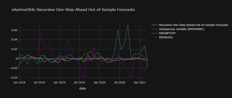
s4arima504c_osaoosf_plot_dic = {
'Recursive One-Step-Ahead Out-of-Sample Forecasts' : np.array(s4arima504c_osaoosf),
'endogenous variable (RMCPANNL)' : RMCPANNL_array_wna}
exogenous_variables = ["RMUNPTOTP", "RMXRUSD."]
for j,k in zip([df.dropna()[i]["yoy1d"].shift(1)[1:].values.tolist()[200:]
for i in exogenous_variables],
exogenous_variables):
s4arima504c_osaoosf_plot_dic[k] = np.array(j).T
s4arima504c_osaoosf_plot_df = pd.DataFrame(
data = s4arima504c_osaoosf_plot_dic,
index = index)
s4arima504c_osaoosf_plot_df.iplot(
theme = "solar", xTitle = "date",
title = "s4arima504c Recursive One-Step-Ahead Out-of-Sample Forecasts")
df2 = df.copy()
s4arima504c_osaoosf_plot_df.tail()
| Recursive One-Step-Ahead Out-of-Sample Forecasts | endogenous variable (RMCPANNL) | RMUNPTOTP | RMXRUSD. | |
| 15/11/2020 | 0.00258 | -0.001 | 0.01044 | -0.0042 |
| 15/12/2020 | 0.00089 | -0.0008 | 0.00959 | 0.00465 |
| 15/01/2021 | -0.0003 | 0.0093 | 0.0163 | -0.0069 |
| 15/02/2021 | -0.0039 | 0.0017 | 0.02746 | -0.0257 |
| 15/03/2021 | -0.0025 | NaN | -0.0195 | -0.0022 |
df2["RMCPANNL", "s4arima504c Recursive OSAOOSF"] = s4arima504c_osaoosf_plot_df["Recursive One-Step-Ahead Out-of-Sample Forecasts"]
df2 = df2.sort_index(axis=1) # This rearranges the columns and merges Fields under the same Instruments.
df2
| Instrument | CLc1 | RMCPANNL | RMGOVBALA | RMUNPTOTP | RMXREUR. | RMXRUSD. | |||||||||||||
| Field | Close Price | Close Price 30D Moving Average | yoy | yoy1d | s4arima504c Recursive OSAOOSF | yoy | yoy1d | raw | yoy | yoy1d | raw | yoy | yoy1d | raw | yoy | yoy1d | raw | yoy | yoy1d |
| 15/01/2001 | 30.05 | 28.535 | 0.09981 | NaN | NaN | 0.399 | NaN | -306.1 | 0.88022 | NaN | 1032.9 | -0.1209 | NaN | 2.4646 | 0.32249 | NaN | 2.62 | 0.42391 | NaN |
| 15/02/2001 | 28.8 | 29.8113 | 0.07816 | -0.0217 | NaN | 0.4 | 0.001 | -601.2 | 0.30158 | -0.5786 | 1032.3 | -0.1373 | -0.0164 | 2.4729 | 0.34244 | 0.01994 | 2.68 | 0.43316 | 0.00924 |
| 15/03/2001 | 26.58 | 28.976 | -0.0423 | -0.1205 | NaN | 0.403 | 0.003 | -865.2 | 0.04746 | -0.2541 | 992.8 | -0.1491 | -0.0117 | 2.4849 | 0.34044 | -0.002 | 2.73 | 0.42188 | -0.0113 |
| 15/04/2001 | 28.2 | 27.25 | -0.0318 | 0.01048 | NaN | 0.375 | -0.028 | -1087.5 | -0.1019 | -0.1494 | 948.4 | -0.1675 | -0.0184 | 2.488 | 0.32956 | -0.0109 | 2.79 | 0.40909 | -0.0128 |
| 15/05/2001 | 28.98 | 27.9327 | 0.0575 | 0.08932 | NaN | 0.374 | -0.001 | -1404.5 | 0.02683 | 0.12874 | 890.8 | -0.1883 | -0.0208 | 2.491 | 0.34598 | 0.01642 | 2.85 | 0.39706 | -0.012 |
| ... | ... | ... | ... | ... | ... | ... | ... | ... | ... | ... | ... | ... | ... | ... | ... | ... | ... | ... | ... |
| 15/10/2020 | 40.92 | 39.4793 | -0.2909 | -0.0379 | -0.0019 | 0.0224 | -0.0021 | -76512 | 1.81579 | -0.0034 | 285.7 | 0.10437 | 0.00959 | 4.8733 | 0.02514 | -0.0004 | 4.14 | -0.0372 | 0.00465 |
| 15/11/2020 | 40.12 | 39.5773 | -0.2836 | 0.00733 | 0.00258 | 0.0214 | -0.001 | -85982 | 1.47431 | -0.3415 | 290.7 | 0.12066 | 0.0163 | 4.8699 | 0.02131 | -0.0038 | 4.12 | -0.0441 | -0.0069 |
| 15/12/2020 | 47.59 | 43.203 | -0.2489 | 0.03465 | 0.00089 | 0.0206 | -0.0008 | -105907 | 1.20275 | -0.2716 | 296.1 | 0.14812 | 0.02746 | 4.8707 | 0.01955 | -0.0018 | 4 | -0.0698 | -0.0257 |
| 15/01/2021 | 52.04 | 48.7013 | -0.1892 | 0.05969 | -0.0003 | 0.0299 | 0.0093 | -112.3 | -0.8426 | -2.0454 | 292.2 | 0.12862 | -0.0195 | 4.8728 | 0.01973 | 0.00018 | 4 | -0.0719 | -0.0022 |
| 15/02/2021 | 59.73 | 53.606 | -0.0281 | 0.16113 | -0.0039 | 0.0316 | 0.0017 | -8430.8 | -0.199 | 0.64362 | 293.5 | 0.14336 | 0.01474 | 4.8741 | 0.01909 | -0.0006 | 4.03 | -0.0799 | -0.008 |
242 rows × 19 columns
As you can see, we are missing the last row of data in df2. We can remedy this by appending it with the last row of s4arima504c_osaoosf_plot_df:
df3 = df2.copy() # just to delimitate from before and after this step.
index_of_interest = s4arima504c_osaoosf_plot_df.tail(1).index[0]
df3 = df3.append(pd.Series(name = index_of_interest))
df3['RMCPANNL', 's4arima504c Recursive OSAOOSF'].loc[index_of_interest] = s4arima504c_osaoosf_plot_df["Recursive One-Step-Ahead Out-of-Sample Forecasts"][-1]
df3
| Instrument | CLc1 | RMCPANNL | RMGOVBALA | RMUNPTOTP | RMXREUR. | RMXRUSD. | |||||||||||||
| Field | Close Price | Close Price 30D Moving Average | yoy | yoy1d | s4arima504c Recursive OSAOOSF | yoy | yoy1d | raw | yoy | yoy1d | raw | yoy | yoy1d | raw | yoy | yoy1d | raw | yoy | yoy1d |
| 15/01/2001 | 30.05 | 28.535 | 0.09981 | NaN | NaN | 0.399 | NaN | -306.1 | 0.88022 | NaN | 1032.9 | -0.1209 | NaN | 2.4646 | 0.32249 | NaN | 2.62 | 0.42391 | NaN |
| 15/02/2001 | 28.8 | 29.8113 | 0.07816 | -0.0217 | NaN | 0.4 | 0.001 | -601.2 | 0.30158 | -0.5786 | 1032.3 | -0.1373 | -0.0164 | 2.4729 | 0.34244 | 0.01994 | 2.68 | 0.43316 | 0.00924 |
| 15/03/2001 | 26.58 | 28.976 | -0.0423 | -0.1205 | NaN | 0.403 | 0.003 | -865.2 | 0.04746 | -0.2541 | 992.8 | -0.1491 | -0.0117 | 2.4849 | 0.34044 | -0.002 | 2.73 | 0.42188 | -0.0113 |
| 15/04/2001 | 28.2 | 27.25 | -0.0318 | 0.01048 | NaN | 0.375 | -0.028 | -1087.5 | -0.1019 | -0.1494 | 948.4 | -0.1675 | -0.0184 | 2.488 | 0.32956 | -0.0109 | 2.79 | 0.40909 | -0.0128 |
| 15/05/2001 | 28.98 | 27.9327 | 0.0575 | 0.08932 | NaN | 0.374 | -0.001 | -1404.5 | 0.02683 | 0.12874 | 890.8 | -0.1883 | -0.0208 | 2.491 | 0.34598 | 0.01642 | 2.85 | 0.39706 | -0.012 |
| ... | ... | ... | ... | ... | ... | ... | ... | ... | ... | ... | ... | ... | ... | ... | ... | ... | ... | ... | ... |
| 15/11/2020 | 40.12 | 39.5773 | -0.2836 | 0.00733 | 0.00258 | 0.0214 | -0.001 | -85982 | 1.47431 | -0.3415 | 290.7 | 0.12066 | 0.0163 | 4.8699 | 0.02131 | -0.0038 | 4.12 | -0.0441 | -0.0069 |
| 15/12/2020 | 47.59 | 43.203 | -0.2489 | 0.03465 | 0.00089 | 0.0206 | -0.0008 | -105907 | 1.20275 | -0.2716 | 296.1 | 0.14812 | 0.02746 | 4.8707 | 0.01955 | -0.0018 | 4 | -0.0698 | -0.0257 |
| 15/01/2021 | 52.04 | 48.7013 | -0.1892 | 0.05969 | -0.0003 | 0.0299 | 0.0093 | -112.3 | -0.8426 | -2.0454 | 292.2 | 0.12862 | -0.0195 | 4.8728 | 0.01973 | 0.00018 | 4 | -0.0719 | -0.0022 |
| 15/02/2021 | 59.73 | 53.606 | -0.0281 | 0.16113 | -0.0039 | 0.0316 | 0.0017 | -8430.8 | -0.199 | 0.64362 | 293.5 | 0.14336 | 0.01474 | 4.8741 | 0.01909 | -0.0006 | 4.03 | -0.0799 | -0.008 |
| 15/03/2021 | NaN | NaN | NaN | NaN | -0.0025 | NaN | NaN | NaN | NaN | NaN | NaN | NaN | NaN | NaN | NaN | NaN | NaN | NaN | NaN |
243 rows × 19 columns
Corresponding Month Model
Many in the industry only focus on the same month of previous years in their predicting models (e.g.: only predict this year's March inflation value with previous March values, similarly so with each month of the year). There is some merit to the thought, as other datapoints may sway our data with irrelevant variables. The reason is that demand/supply profiles might be different each month of the day and it would be incorrect to compare months in a continuous series (i.e.: January to February et cetera (etc.)). To do so, we can exploit the SARIMA model and only use Seasonal AutoRegressive variables (in addition to our exogenous variables):
1st: Let's check the best SAMIMA model with ARMA(0,0) imposed:
test0_df, test0_lowest = Reg_Perm_Table(p = [0])
# To save data out:
pickle_out = open("Regression_Permutation_Table0.pickle","wb")
pickle.dump((test0_df, test0_lowest), pickle_out)
pickle_out.close()
# To load data in:
# pickle_in = open("Regression_Permutation_Table0.pickle","rb") # ' rb ' stand for 'read bytes'.
# test0_df, test0_lowest = pickle.load(pickle_in)
# pickle_in.close() # We ought to close the file we opened to allow any other programs access if they need it.
test0_df[test0_df.index.str.contains("sarima0,0,0")]
| AIC | AICC | BIC | HQIC | MSE | SSE | |
| sarima0,0,0,0,0,0,12,c,exo=('CLc1',) | -1656.6 | -1656.5 | -1646.2 | -1652.4 | 5.6E-05 | 0.01333 |
| sarima0,0,0,0,0,0,12,c,exo=('RMGOVBALA',) | -1656.3 | -1656.2 | -1645.8 | -1652.1 | 5.6E-05 | 0.01335 |
| sarima0,0,0,0,0,0,12,c,exo=('RMUNPTOTP',) | -1657.4 | -1657.2 | -1646.9 | -1653.1 | 5.6E-05 | 0.01329 |
| sarima0,0,0,0,0,0,12,c,exo=('RMXREUR.',) | -1665 | -1664.9 | -1654.6 | -1660.8 | 5.4E-05 | 0.01287 |
| sarima0,0,0,0,0,0,12,c,exo=('RMXRUSD.',) | -1660.1 | -1660 | -1649.7 | -1655.9 | 5.5E-05 | 0.01313 |
| ... | ... | ... | ... | ... | ... | ... |
| sarima0,0,0,4,0,4,12,c,exo=('CLc1', 'RMGOVBALA', 'RMUNPTOTP', 'RMXRUSD.') | -1625.7 | -1623.8 | -1577 | -1606.1 | 5.4E-05 | 0.01283 |
| sarima0,0,0,4,0,4,12,c,exo=('CLc1', 'RMGOVBALA', 'RMXREUR.', 'RMXRUSD.') | -1632.4 | -1630.5 | -1583.7 | -1612.7 | 5.2E-05 | 0.01249 |
| sarima0,0,0,4,0,4,12,c,exo=('CLc1', 'RMUNPTOTP', 'RMXREUR.', 'RMXRUSD.') | -1669.6 | -1667.7 | -1620.9 | -1650 | 0.00005 | 0.01196 |
| sarima0,0,0,4,0,4,12,c,exo=('RMGOVBALA', 'RMUNPTOTP', 'RMXREUR.', 'RMXRUSD.') | -1636.1 | -1634.2 | -1587.4 | -1616.5 | 5.2E-05 | 0.0124 |
| sarima0,0,0,4,0,4,12,c,exo=('CLc1', 'RMGOVBALA', 'RMUNPTOTP', 'RMXREUR.', 'RMXRUSD.') | -1633.8 | -1631.6 | -1581.6 | -1612.8 | 5.2E-05 | 0.01241 |
775 rows × 6 columns
test0_df[test0_df.index.str.contains("sarima0,0,0")].nsmallest(1, 'SSE').index
Index(['sarima0,0,0,3,0,0,12,c,exo=('RMUNPTOTP', 'RMXREUR.', 'RMXRUSD.')'], dtype='object')
Note that our Reg_Perm_Table function's default Seasonal parameters (P and Q) range from 0 to 5 and that the optimum (i.e.: lowest SSE producing one) is lower than 5; this would indicate that we may very well have our optimal SAMIMA model with ARMA(0,0) imposed
exogenous_variables = ['RMUNPTOTP', 'RMXREUR.', 'RMXRUSD.']
s3arima000c = ARIMA(
endog = np.array(df.dropna()["RMCPANNL"]["yoy1d"][1:].values.tolist())[0:200],
exog = np.array([df.dropna()[i]["yoy1d"].shift(1)[1:].values.tolist()[0:200]
for i in exogenous_variables]).T,
order = (0, 0, 0),
trend = "c",
seasonal_order = (3, 0, 0, 12))
s3arima000c_isf = s3arima000c.fit() # 'isf' for in-sample-fit
s3arima000c_isf_plot_dic = {
'residuals' : s3arima000c_isf.resid,
'fitted values' : s3arima000c_isf.fittedvalues,
'endogenous variable (RMCPANNL)' : np.array(
df.dropna()["RMCPANNL"]["yoy1d"][1:].values.tolist())[0:200]}
for j,k in zip([df.dropna()[i]["yoy1d"].shift(1)[1:].values.tolist()[0:200]
for i in exogenous_variables],
exogenous_variables):
s3arima000c_isf_plot_dic[k] = np.array(j).T
s3arima000c_isf_plot_df = pd.DataFrame(data = s3arima000c_isf_plot_dic,
index = df.dropna()["RMCPANNL"]["yoy1d"][1:][0:200].index)
s3arima000c_isf_plot_df.iplot(theme = "solar",
title = "s3arima000c in-sample-forecasts model fit",
xTitle = "date")
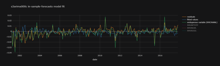
s3arima000c_osaoosf = []
for t in range(200, len(df.dropna()["RMCPANNL"]["yoy1d"][1:])):
if t%10 == 0 : print("Our code has created one-step-ahead out-of-sample forecasts from 200 to " str(t)) # This line is to see the progression of our code.
s3arima000c = ARIMA(
endog = np.array(df.dropna()["RMCPANNL"]["yoy1d"][1:].values.tolist())[0:t-1],
exog = np.array([df.dropna()[i]["yoy1d"].shift(1)[1:].values.tolist()[0:t-1]
for i in exogenous_variables]).T,
order = (0, 0, 0),
trend = "c",
seasonal_order = (3, 0, 0, 12))
s3arima000c_isf = s3arima000c.fit() # 'isf' for in-sample-fit
s3arima000c_osaoosf.append( # 'osaoosf' as in One-Step-Ahead Out-of-Sample Forecasts
s3arima000c_isf.forecast(
exog = np.array([df.dropna()[i]["yoy1d"].shift(1)[1:].values.tolist()[t]
for i in exogenous_variables]).T)[0])
200
210
220
230
Let's save our data in s3arima000c_osaoosf:
# saving data into a pickle file::
pickle_out = open("s3arima000c_osaoosf.pickle","wb")
pickle.dump(s3arima000c_osaoosf, pickle_out)
pickle_out.close()
# # loading data from the pickle file:
# pickle_in = open('s3arima000c_osaoosf.pickle','rb') # ' rb ' stand for 'read bytes'.
# s3arima000c_osaoosf = pickle.load(pickle_in)
# pickle_in.close() # We ought to close the file we opened to allow any other programs access if they need it.
# add a month to the index:
index_in_qu = df.dropna()["RMCPANNL"]["yoy1d"][1:][200:].index
index = [i for i in index_in_qu][1:] + [
str(datetime.strptime(str(pd.to_datetime(
[str(i) for i in index_in_qu])[-1].replace(
month = pd.to_datetime(str(df.index[-1])).month+1)),
'%Y-%m-%d %H:%M:%S'))[:10]]
s3arima000c_osaoosf_plot_dic = {
'Recursive One-Step-Ahead Out-of-Sample Forecasts' : np.array(s3arima000c_osaoosf),
'endogenous variable (RMCPANNL)' : np.append(
np.array(df.dropna()["RMCPANNL"]["yoy1d"][1:].values.tolist())[200 + 1:],
[np.nan])}
for j,k in zip([df.dropna()[i]["yoy1d"].shift(1)[1:].values.tolist()[200:]
for i in exogenous_variables],
exogenous_variables):
s3arima000c_osaoosf_plot_dic[k] = np.array(j).T
s3arima000c_osaoosf_plot_df = pd.DataFrame(
data = s3arima000c_osaoosf_plot_dic,
index = index)
s3arima000c_osaoosf_plot_df.iplot(
theme = "solar", xTitle = "date",
title = "s3arima000c Recursive One-Step-Ahead Out-of-Sample Forecasts")
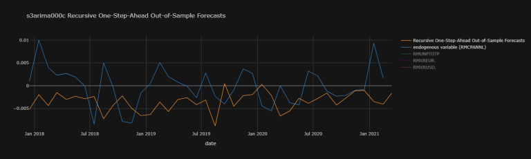
for i,j in zip([s3arima000c_osaoosf_plot_df], [s4arima504c_osaoosf_plot_df]):
s3arima000c_resid = i["endogenous variable (RMCPANNL)"] - i["Recursive One-Step-Ahead Out-of-Sample Forecasts"][:-1]
s4arima504c_resid = j["endogenous variable (RMCPANNL)"] - j["Recursive One-Step-Ahead Out-of-Sample Forecasts"][:-1]
s3arima000c_sse = (s3arima000c_resid**2).sum()
s4arima504c_sse = (s4arima504c_resid**2).sum()
print(s3arima000c_sse, s4arima504c_sse)
0.0013175028279920704 0.0012139805753142835
From the two SSE values above, we can determine that our s4arima504c model is the better of the two.
Conclusion
The fact that a model with seasonal components (SARIMA(5,0,4)(4,0,0)1212) was the optimal one (even before we investigate Corresponding Month Models) suggests that there was a lot of information in corresponding months in previous years. As a matter of fact, even the directly previous months' coefficients seemed of little relevance. Indeed, s4arima504c_fit P-values of these cofactors from lag 1 to 4 (ar.L1 to ar.L4) never went below 0.1; i.e.: they were never statistically significant. The 5th lag however (ar.L5, with value 0.2342) had a P-value lower than 0.05, suggesting it to be statistically significant at the 5% Confidence Level (CL). Moving Average elements (ma.L1 to ma.L4) never showed statistical significance (as per their P-values). (Statistical significance is only really considered at the 10% CL, when the P-value is lower than 0.1.)
Seasonal coefficients 1 to 3 (ar.S.L12 to ar.S.L36) proved significant at the 5% CL. The 4th (ar.S.L48) did not.
It would be interesting to look at a non-consecutive lags model with only ar.L5 & ar.S.L12 to ar.S.L36 and investigate it's out-of-sample one-step-ahead forecasts as a back-test.
Additionally, what make this model interesting is that one can use it for more than one-step-ahead forecasts depending on the frequency of exogenous data provision. Say that the exogenous RMXRUSD variable is only published on the 30th of the month (showing data for the 15th of that month); than one can use data published a month prior to forecast two-steps-ahead, alleviating this issue - although not solving it per se (by itself).
Romanian inflation is a particular case study. High inflation levels a the start of our data-set might have skewed results significantly. A look at models such as the ones above in predicting other countries' inflation levels could be more fruitful. Alternatively, looking into more differenced data could be equally interesting. (Indeed, using Stationarity_Table with more differenced data seem to yield more stationary data.)
References
Model Specifications
- Time Series Forecasting with SARIMA in Python
- Problem defining ARIMA order
- Model selection by The Akaike’s Information Criterion (AIC) what is common practice?
- pmdarima Python Library
- In general, choosing the order of the model (e.g. p, q and P, Q) via information criteria is a good idea, but it is not a good idea to choose the differencing order (d or D) that way.
- Time Series Talk : Seasonal ARIMA Model
Model Performance
- How to find relative influence of Exogenous variables from a ARIMA model?
- Out of sample risk estimates are the gold standard for performance evaluation
Academic Refferences
- FORECASTING INFLATION THROUGH ECONOMETRIC MODELS: AN EMPIRICAL STUDY ON PAKISTANI DATA
- Quarterly inflation rate target and forecasts in Romania
- THE EVOLUTION OF CONSUMER PRICES IN JANUARY 202
- Concepte de bază și definiții
Multi-Processing
- Python Multiprocessing Tutorial: Run Code in Parallel Using the Multiprocessing Module
- Parallel Processing in Python – A Practical Guide with Examples
- Multiprocessing in Python on Windows and Jupyter/Ipython — Making it work