Authors:

In this article, we'll create an application that will display statistics of an instrument (e.g.: the foreign exchange (fx) pair) immediately (precise up to a second) after a press release of interest (e.g.: United States' Consumer Price Index (CPI) or US Non Farm Payroll) that can run in CodeBook. This way, you can have such a view on one side of your Workspace, and any other app of choice on the other. We'll display a live, interactive graph of the tick data, and a static table of the historical report data. We will use LSEG Refinitiv's Datastream DSWS API (Application Programming Interface) to collect historical report data; this API has such data going back donkey's years (sometimes back to the 1950s) and it has a navigator in which you can find the relevant report of choice, as outlined brilliantly in Jirapongse's article here. For the tick data, we will use LSEG's Refinitiv Data API; it - however - does not natively allow access to tick data going that far back (only for the past 3 to 5 months). I will endeavour to update this article in the future with use of the LSEG Refinitiv TRTH (Refinitiv Tick History) REST (REpresentational State Transfer) API that may allow us access to tick data further back in time.
Some Imports to start with
Python works with libraries that one can import to use functionalities that are not natively supported but the coding language.
# The ' from ... import ' structure here allows us to only import the module ' python_version ' from the library ' platform ':
import platform
from platform import python_version # The ` python_version ` will allow us to display our evvironment details to help you replicate this code.
print("This code runs on Python version " + python_version() + " in " + platform.architecture()[0])
This code runs on Python version 3.8.2 in 32bit
import pandas as pd # `pandas` is a widely-used Python library that allows us to manipulate data-frames.
import numpy as np # `numpy` is a widely-used Python library that allows us to manipulate number arrays.
import datetime # `datetime` allows us to manipulate time as it it was data points
import warnings # Some data manipulations throw warnings that polute the display we'll build; it is thus best to remove them for now; this `warnings` library will allow us to do just that.
Polls / Estimates Data
We need to gather our economic estimates data to calculate the surprise seen in the metric of interest (e.g.: US Inflation) straight after the release of a report (e.g.: US Inflation Report). Since Refinitiv's DataStream Web Services (DSWS) allows for access to the most accurate and wholesome economic database (DB), naturally it is more than appropriate. We can access DSWS via the Python library "DatastreamDSWS" that can be installed simply by using pip installpip install.
Make sure to entre correct DataStream credentials
import DatastreamDSWS as DSWS
# The username and password is placed in a text file so that it may be used in this code without showing it itself.
dsws_username = open("Datastream_username.txt", "r")
dsws_password = open("Datastream_password.txt", "r")
ds = DSWS.Datastream(username = str(dsws_username.read()), password = str(dsws_password.read()))
# It is best to close the files we opened in order to make sure that we don't stop any other services/programs from accessing them if they need to.
dsws_username.close()
dsws_password.close()
We need to find out exactly when (date and time) the last report was released. In our example, we looked at CPI in the US. This is reported retroactively (i.e.: when a press release with CPI figures are published, they inform readers of what the CPI was in past dates). What we were interested in up to now were the datapoints themselves; but now we'll look at FX changes at time of press release. For the sake of this example, let's say it was last released on 11-May-2022 at 13:34. That's what the TREL1 is there for.
startDate = '2020-06-01'
_reportActual = ds.get_data(
tickers = 'USCONPRCE', # USCONPRCE for US CPI and USPENOACO for NonFarmPayrolls.
fields = ['X', 'TREL1', 'DREL1'],
start = startDate,
freq = 'M')
DSWS returns dataframes with MultiIndex columns.
_reportActual.columns
MultiIndex([('USCONPRCE', 'X'),
('USCONPRCE', 'TREL1'),
('USCONPRCE', 'DREL1')],
names=['Instrument', 'Field'])
While this is extremely useful for data analytics, it'll better for us to flatten it to a single dimention
_reportActualColumns = [[_reportActual.columns[i][j] for i in range(len(_reportActual.columns))] for j in range(len(_reportActual.columns[0]))]
reportActualColumns = [k + "_" + l for k, l in zip(_reportActualColumns[0], _reportActualColumns[1])]
Now let's tidy our data up in teh reportActual data-frame:
reportActual = pd.DataFrame(
data=_reportActual.values,
columns=reportActualColumns,
index=_reportActual.index)
reportActual
| USCONPRCE_X | USCONPRCE_TREL1 | USCONPRCE_DREL1 | |
| Dates | |||
| 15/06/2020 | 257.217 | 12:31:00 | 14/07/2020 |
| 15/07/2020 | 258.543 | 12:39:38 | 12/08/2020 |
| 15/08/2020 | 259.58 | 12:32:00 | 11/09/2020 |
| ... | |||
| 15/03/2022 | 287.708 | 12:36:30 | 12/04/2022 |
| 15/04/2022 | 288.663 | 12:36:30 | 11/05/2022 |
| 15/05/2022 | 291.474 | 12:36:30 | 10/06/2022 |
| 15/06/2022 | NaN | None | None |
Let's create a function that does that for us
def GetDSWSDataAndFalattenColumns(tickers, fields, freq, start=startDate, adjustment=0):
'''GetDSWSDataAndFalattenColumns V1.0:
One needs a LSEG Refinitiv's Datastream DSWS API(https://developers.refinitiv.com/en/api-catalog/eikon/datastream-web-service) and a working account/license.
It works by collecting DSWS data for the `tickers`, `fields`, `freq` and `start` and flattens the MultiIndex columns it usually comes out with.
Dependencies
----------
Python library 'pandas' version 1.2.4
Python library 'DatastreamDSWS' as DSWS (!pip install DatastreamDSWS)
Parameters
----------
`tickers`, `fields`, `freq` and `start`: str
For information on these function parameters, please run:
import DatastreamDSWS as DSWS
ds = DSWS.Datastream(username = "USERNAME", password = "PASSWORD"))
help(ds)
adjustment: int
I found that someties the column number was not nessesarily correct, so you can adjust it here.
Default: adjustment=0
Returns
-------
pandas dataframe
'''
df = ds.get_data(tickers=tickers, fields=fields, start=start, freq=freq)
columns = [[df.columns[i][j] for i in range(len(df.columns))]
for j in range(len(df.columns[0]) + adjustment)]
columns = [k + "_" + l for k, l in zip(columns[0], columns[1])]
df = pd.DataFrame(data=df.values, columns=columns, index=df.index)
return df
reportPoll = GetDSWSDataAndFalattenColumns(
tickers = 'US&CPNM.F',
fields = "X",
freq = 'M')
reportSurprise = GetDSWSDataAndFalattenColumns(
tickers = 'US&CPNS.F',
fields = 'X',
freq = 'M')
reportNames = ds.get_data(
tickers = 'USCONPRCE,US&CPNM.F,US&CPNS.F',
fields = ['NAME'],
kind = 0) # `kind = 0` is for static data, i.e.: data that is not meant to change through time, like the name of a company.
reportNames
| Instrument | Datatype | Value | Dates | |
| 0 | USCONPRCE | NAME | US CPI - ALL URBAN: ALL ITEMS SADJ | 24/06/2022 |
| 1 | US&CPNM.F | NAME | US CPI INDEX, NSA-MEDIAN NADJ | 24/06/2022 |
| 2 | US&CPNS.F | NAME | US CPI INDEX, NSA-SURPRISE NADJ | 24/06/2022 |
reportActual
| USCONPRCE_X | USCONPRCE_TREL1 | USCONPRCE_DREL1 | |
| Dates | |||
| 15/06/2020 | 257.217 | 12:31:00 | 14/07/2020 |
| 15/07/2020 | 258.543 | 12:39:38 | 12/08/2020 |
| 15/08/2020 | 259.58 | 12:32:00 | 11/09/2020 |
| ... | |||
| 15/03/2022 | 287.708 | 12:36:30 | 12/04/2022 |
| 15/04/2022 | 288.663 | 12:36:30 | 11/05/2022 |
| 15/05/2022 | 291.474 | 12:36:30 | 10/06/2022 |
| 15/06/2022 | NaN | None | None |
# Let's put all this data together
reportDf = pd.merge(
pd.merge(
reportActual, reportPoll, left_index=True, right_index=True),
reportSurprise, left_index=True, right_index=True)
reportDf.dropna()
# Let's create a plot data-frame to get a nice looking graph,
plotDf = reportDf.dropna()[['USCONPRCE_X', 'US&CPNM.F_X', 'US&CPNS.F_X']]
plotDf.index = reportDf.dropna().USCONPRCE_DREL1
# Unfortunutally, some of the data provided are of different data types. We can homogenise it for easier proccessing:
for i in plotDf.columns:
plotDf[i] = [float(j) for j in plotDf[i].to_list()]
Let's plot our data to visualise it; we can use plotly with the pd.options.plotting.backend function:
pd.options.plotting.backend = "plotly" # https://plotly.com/python/pandas-backend/
plotDf.dropna().plot(
title='USCONPRCE (US CPI - ALL URBAN: ALL ITEMS SADJ), US&CPNM.F (US CPI INDEX, NSA-MEDIAN NADJ), US&CPNS.F (US CPI INDEX, NSA-SURPRISE NADJ)',
template='plotly_dark') # need `pip install nodejs` & the `@jupyterlab/plotly-extension` if in Jupyter Lab outside CodeBook.
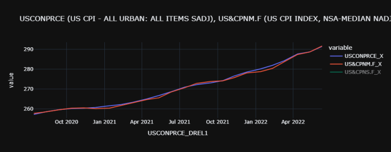
reportDf.dropna()
| USCONPRCE_X | USCONPRCE_TREL1 | USCONPRCE_DREL1 | US&CPNM.F_X | US&CPNS.F_X | |
| Dates | |||||
| 15/06/2020 | 257.217 | 12:31:00 | 14/07/2020 | 257.733 | 0.064 |
| 15/07/2020 | 258.543 | 12:39:38 | 12/08/2020 | 258.51 | 0.591 |
| 15/08/2020 | 259.58 | 12:32:00 | 11/09/2020 | 259.518 | 0.4 |
| ... | |||||
| 15/03/2022 | 287.708 | 12:36:30 | 12/04/2022 | 287.41 | 0.094 |
| 15/04/2022 | 288.663 | 12:36:30 | 11/05/2022 | 288.654 | 0.455 |
| 15/05/2022 | 291.474 | 12:36:30 | 10/06/2022 | 291.661 | 0.635 |
Tick Data
In the cell bellow, we import the Python library os, then we use it to point to the path where our Refinitiv Credentials are; we need this file in order to authenticate ourselves to the Refinitiv data services and collect data. You can find out more on this here, and a copy of the Configuration file here.
import os # This module provides a portable way of using operating system dependent functionality.
os.environ["RD_LIB_CONFIG_PATH"] = "C:\\Example.DataLibrary.Python-main\\Example.DataLibrary.Python-main\\Configuration" # Here we point to the path to our configuration file.
# To install the RD library, you may need to run `!pip install refinitiv-data` in Jupyter Lab/Notebook1.
import refinitiv.data as rd # pip install httpx==0.21.3
rd.open_session("desktop.workspace") # Send info to the Refinitiv system (i.e.: the API)
# rd.open_session("desktop.workspace") # If running this code outside CodeBook. You can also try "platform.rdp"
# rd.open_session("") # If running this code within CodeBook. # 'DEFAULT_CODE_BOOK_APP_KEY' is also often used in CodeBook. More on CodeBook here: https://www.refinitiv.com/content/dam/marketing/en_us/documents/fact-sheets/codebook.pdf
# Let's get the last report's release date and time:
lastReportTime = datetime.datetime.strptime(reportDf.dropna().USCONPRCE_DREL1[-1] + "T" + reportDf.dropna().USCONPRCE_TREL1[-1], "%Y-%m-%dT%H:%M:%S")
# Let's collect tick-data for the next 15 minutes after that last report's release:
toTime = lastReportTime + datetime.timedelta(minutes=15) # This object will be the time we're collecting tick-fx-data until.
print(f"The last report was on {lastReportTime.strftime('%Y-%m-%dT%H:%M:%S')} and we'll get FX data till {toTime.strftime('%Y-%m-%dT%H:%M:%S')}")
The last report was on 2022-06-10T12:36:30 and we'll get FX data till 2022-06-10T12:51:30
# Now that we have the date and time for which we would like to collect data, we can send our tick data request:
fxDf = rd.content.historical_pricing.events.Definition(
universe="GBP=",
fields=['BID', 'ASK', 'MID_PRICE'], # ['TR.BIDPRICE', 'TR.BIDPRICE.date']
start=lastReportTime.strftime("%Y-%m-%dT%H:%M:%S"),
end=toTime.strftime("%Y-%m-%dT%H:%M:%S")).get_data().data.df
fxDf.drop('EVENT_TYPE', inplace=True, axis=1) # This is a column of str's, which can mess up with the maths and plots we want to do
for i in fxDf.columns:
fxDf[i] = fxDf[i].astype(float) # `MID_PRICE` data is returned in str form, we would like it in float so that we can do some maths with it.
# Let's go through our calculations:
fxDf['RatioChangeSince' + lastReportTime.strftime("%Y-%m-%dT%H:%M:%S")] = (
fxDf['MID_PRICE'] - fxDf['MID_PRICE'][0])/fxDf['MID_PRICE'][0]
fxDf['%ChangeSince' + lastReportTime.strftime("%Y-%m-%dT%H:%M:%S")] = fxDf[
'RatioChangeSince' + lastReportTime.strftime("%Y-%m-%dT%H:%M:%S")]*100
fxDf['Average%ChangeSince' + lastReportTime.strftime("%Y-%m-%dT%H:%M:%S")] = [
np.average(fxDf['%ChangeSince' + lastReportTime.strftime("%Y-%m-%dT%H:%M:%S")].iloc[0:i]) for i in range(len(fxDf))]
fxDf['StandardDeviationOf%ChangeSince' + lastReportTime.strftime("%Y-%m-%dT%H:%M:%S")] = [
fxDf['%ChangeSince' + lastReportTime.strftime("%Y-%m-%dT%H:%M:%S")].iloc[0:i].std() for i in range(len(fxDf))]
fxDf['UpperBoundOfStandardDeviationOf%ChangeSince' + lastReportTime.strftime("%Y-%m-%dT%H:%M:%S")] = [
fxDf['Average%ChangeSince' + lastReportTime.strftime("%Y-%m-%dT%H:%M:%S")].iloc[i] +
fxDf['StandardDeviationOf%ChangeSince' + lastReportTime.strftime("%Y-%m-%dT%H:%M:%S")].iloc[i]
for i in range(len(fxDf))]
fxDf['LowerBoundOfStandardDeviationOf%ChangeSince' + lastReportTime.strftime("%Y-%m-%dT%H:%M:%S")] = [
fxDf['Average%ChangeSince' + lastReportTime.strftime("%Y-%m-%dT%H:%M:%S")].iloc[i] -
fxDf['StandardDeviationOf%ChangeSince' + lastReportTime.strftime("%Y-%m-%dT%H:%M:%S")].iloc[i]
for i in range(len(fxDf))]
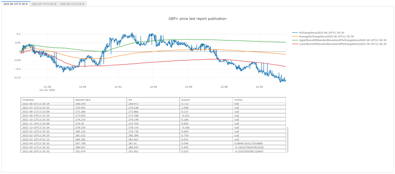
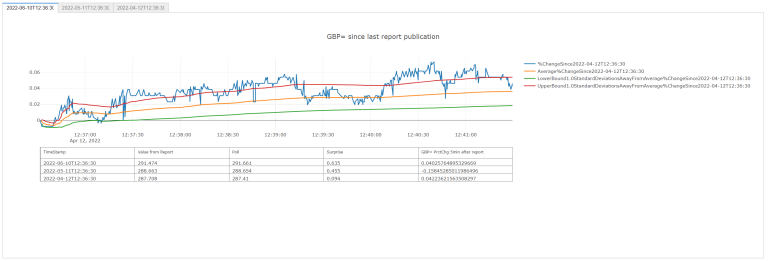
fxDf
| GBP= | BID | ASK | MID_PRICE | RatioChangeSince2022-06-10T12:36:30 | %ChangeSince2022-06-10T12:36:30 | Average%ChangeSince2022-06-10T12:36:30 | StandardDeviationOf%ChangeSince2022-06-10T12:36:30 | UpperBoundOfStandardDeviationOf%ChangeSince2022-06-10T12:36:30 | LowerBoundOfStandardDeviationOf%ChangeSince2022-06-10T12:36:30 |
| Timestamp | |||||||||
| 2022-06-10 12:36:30.258000+00:00 | 1.2418 | 1.2422 | 1.242 | 0 | 0 | NaN | NaN | NaN | NaN |
| 2022-06-10 12:36:30.260000+00:00 | 1.2419 | 1.242 | 1.24195 | -0.00004 | -0.004026 | 0 | NaN | NaN | NaN |
| ... | ... | ... | ... | ... | ... | ... | ... | ... | ... |
| 2022-06-10 12:51:29.168000+00:00 | 1.2399 | 1.24 | 1.23995 | -0.001651 | -0.165056 | -0.016765 | 0.070156 | 0.053391 | -0.086921 |
| 2022-06-10 12:51:29.960000+00:00 | 1.2398 | 1.2402 | 1.24 | -0.00161 | -0.161031 | -0.016834 | 0.070212 | 0.053378 | -0.087046 |
2149 rows × 9 columns
# Now let's have a quick plot to look at our work:
fxPlotDf = fxDf.drop(
['BID', 'ASK', 'MID_PRICE',
'StandardDeviationOf%ChangeSince' + lastReportTime.strftime("%Y-%m-%dT%H:%M:%S"),
'RatioChangeSince' + lastReportTime.strftime("%Y-%m-%dT%H:%M:%S")], axis=1)
fxPlotDf.plot(
title=f'GBP= since last report publication at {lastReportTime.strftime("%Y-%m-%dT%H:%M:%S")}',
template='plotly_dark') # need `pip install nodejs` & the `@jupyterlab/plotly-extension` if in Jupyter Lab outside CodeBook.
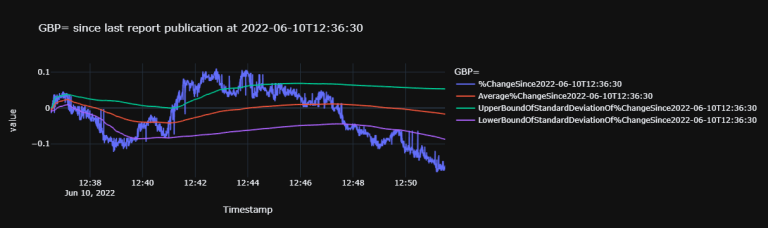
fxPlotDf
| GBP= | %ChangeSince2022-06-10T12:36:30 | Average%ChangeSince2022-06-10T12:36:30 | UpperBoundOfStandardDeviationOf%ChangeSince2022-06-10T12:36:30 | LowerBoundOfStandardDeviationOf%ChangeSince2022-06-10T12:36:30 |
| Timestamp | ||||
| 2022-06-10 12:36:30.258000+00:00 | 0 | NaN | NaN | NaN |
| 2022-06-10 12:36:30.260000+00:00 | -0.004026 | 0 | NaN | NaN |
| 2022-06-10 12:36:30.635000+00:00 | -0.012077 | -0.002013 | 0.000834 | -0.00486 |
| 2022-06-10 12:36:30.740000+00:00 | 0 | -0.005368 | 0.000782 | -0.011517 |
| 2022-06-10 12:36:31.099000+00:00 | 0 | -0.004026 | 0.001668 | -0.009719 |
| ... | ... | ... | ... | ... |
| 2022-06-10 12:51:29.168000+00:00 | -0.165056 | -0.016765 | 0.053391 | -0.086921 |
| 2022-06-10 12:51:29.960000+00:00 | -0.161031 | -0.016834 | 0.053378 | -0.087046 |
2149 rows × 4 columns
df = pd.DataFrame(
data=reportDf.dropna()[['USCONPRCE_X', 'US&CPNM.F_X', 'US&CPNS.F_X']].values,
index=[reportDf.dropna()['USCONPRCE_DREL1'].iloc[i] + 'T' + reportDf.dropna()['USCONPRCE_TREL1'].iloc[i]
for i in range(len(reportDf.dropna()))],
columns=['Reported Value', 'Poll', 'Surprise'])
df
|
Reported Value | Poll | Surprise |
| 2020-07-14T12:31:00 | 257.217 | 257.733 | 0.064 |
| 2020-08-12T12:39:38 | 258.543 | 258.51 | 0.591 |
| 2020-09-11T12:32:00 | 259.58 | 259.518 | 0.4 |
| ... | |||
| 2022-04-12T12:36:30 | 287.708 | 287.41 | 0.094 |
| 2022-05-11T12:36:30 | 288.663 | 288.654 | 0.455 |
| 2022-06-10T12:36:30 | 291.474 | 291.661 | 0.635 |
For historical FX data, we will have to use the ek library and authenticate ourselves to it. This library will only work with Workspace/Eikon running in the background or in CodeBook.
dfs = {'fromTime': [], 'toTime': [], 'fxDf': [], 'prctChg': [], 'fxPlotDf' : []} # In this dictionary, there will be a list full of all the datafames collected 7 the percent change that we're after
for i in range(len(reportDf.dropna())):
_lastReportTime = datetime.datetime.strptime( # The `_` in front of variables usually denotes that they are temporary and can be over written in the future, e.g.: over every loop.
reportDf.dropna().USCONPRCE_DREL1[i] + "T" + reportDf.dropna().USCONPRCE_TREL1[i], "%Y-%m-%dT%H:%M:%S") # We are writing time codes here in the Refinitiv default way for consistency's sake.
_toTime = _lastReportTime + datetime.timedelta(minutes=15) # This object will be the time we're collecting tick-fx-data until.
try: # There isn't nessesarily going to be all the data what we're after, going back as far as we want; that's why we're going through a try loop.
_fxDf = rd.content.historical_pricing.events.Definition(
universe="GBP=",
fields=['MID_PRICE'], # ['TR.BIDPRICE', 'TR.BIDPRICE.date']
start=_lastReportTime.strftime("%Y-%m-%dT%H:%M:%S"),
end=_toTime.strftime("%Y-%m-%dT%H:%M:%S")).get_data().data.df
print(f"We'll get data from {_lastReportTime.strftime('%Y-%m-%dT%H:%M:%S')} till {_toTime.strftime('%Y-%m-%dT%H:%M:%S')}") # This line is here so that we can tell exactly what data we're calling for.
_fxDf.drop('EVENT_TYPE', inplace=True, axis=1) # This is a column of str's, which can mess up with the maths and plots we want to do
for i in _fxDf.columns:
_fxDf[i] = _fxDf[i].astype(float) # `MID_PRICE` data is returned in str form, we would like it in float so that we can do some maths with it.
_fxDf['%ChangeSince' + _lastReportTime.strftime("%Y-%m-%dT%H:%M:%S")] = ((
_fxDf['MID_PRICE'] - _fxDf['MID_PRICE'][0])/_fxDf['MID_PRICE'][0])*100
_fxDf['Average%ChangeSince' + _lastReportTime.strftime("%Y-%m-%dT%H:%M:%S")] = [
np.average(_fxDf['%ChangeSince' + _lastReportTime.strftime("%Y-%m-%dT%H:%M:%S")].iloc[0:i])
for i in range(len(_fxDf))]
_fxDf['StandardDeviationOf%ChangeSince' + _lastReportTime.strftime("%Y-%m-%dT%H:%M:%S")] = [
_fxDf['%ChangeSince' + _lastReportTime.strftime("%Y-%m-%dT%H:%M:%S")].iloc[0:i].std()
for i in range(len(_fxDf))]
_fxDf['UpperBoundOfStandardDeviationOf%ChangeSince' + _lastReportTime.strftime("%Y-%m-%dT%H:%M:%S")] = [
_fxDf['Average%ChangeSince' + _lastReportTime.strftime("%Y-%m-%dT%H:%M:%S")].iloc[i] +
_fxDf['StandardDeviationOf%ChangeSince' + _lastReportTime.strftime("%Y-%m-%dT%H:%M:%S")].iloc[i]
for i in range(len(_fxDf))]
_fxDf['LowerBoundOfStandardDeviationOf%ChangeSince' + _lastReportTime.strftime("%Y-%m-%dT%H:%M:%S")] = [
_fxDf['Average%ChangeSince' + _lastReportTime.strftime("%Y-%m-%dT%H:%M:%S")].iloc[i] -
_fxDf['StandardDeviationOf%ChangeSince' + _lastReportTime.strftime("%Y-%m-%dT%H:%M:%S")].iloc[i]
for i in range(len(_fxDf))]
_fxPlotDf = _fxDf.drop(
['MID_PRICE',
'StandardDeviationOf%ChangeSince' + _lastReportTime.strftime("%Y-%m-%dT%H:%M:%S")],
axis=1)
dfs['fromTime'].append(_lastReportTime.strftime('%Y-%m-%dT%H:%M:%S'))
dfs['toTime'].append(_toTime.strftime("%Y-%m-%dT%H:%M:%S"))
dfs['fxDf'].append(_fxDf)
dfs['prctChg'].append(_fxDf['%ChangeSince' + _lastReportTime.strftime("%Y-%m-%dT%H:%M:%S")].iloc[-1])
dfs['fxPlotDf'].append(_fxPlotDf)
except:
pass
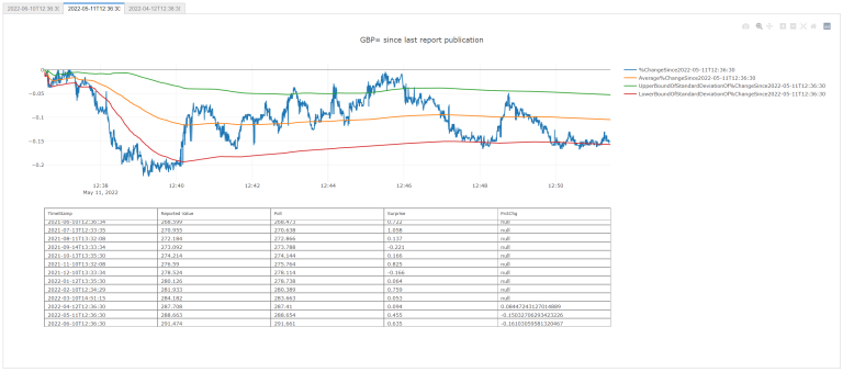
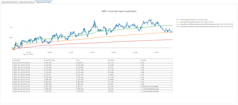
We'll get data from 2022-04-12T12:36:30 till 2022-04-12T12:51:30
We'll get data from 2022-05-11T12:36:30 till 2022-05-11T12:51:30
We'll get data from 2022-06-10T12:36:30 till 2022-06-10T12:51:30
# In order to find out the % change of our tick data over the chosen window, we need to only add data as far back as we have this tick data. The `NaN` will be there to complete the dataframe.
prctChg = [np.nan for i in range(len(df) - len(dfs['prctChg']))] # `NaN`s in question.
for i in dfs['prctChg']: prctChg.append(i) # Now we can append with the data we actually have.
df['PrctChg'] = prctChg # And now we can add the data to our dataframe.
df.insert(0, 'TimeStamp', df.index) # This is only just to have a column with Timestamps that show up in the table in our app displayed at the end.
df
| TimeStamp | Reported Value | Poll | Surprise | PrctChg | |
| 2020-07-14T12:31:00 | 2020-07-14T12:31:00 | 257.217 | 257.733 | 0.064 | NaN |
| 2020-08-12T12:39:38 | 2020-08-12T12:39:38 | 258.543 | 258.51 | 0.591 | NaN |
| 2020-09-11T12:32:00 | 2020-09-11T12:32:00 | 259.58 | 259.518 | 0.4 | NaN |
| ... | |||||
| 2022-04-12T12:36:30 | 2022-04-12T12:36:30 | 287.708 | 287.41 | 0.094 | 0.084472 |
| 2022-05-11T12:36:30 | 2022-05-11T12:36:30 | 288.663 | 288.654 | 0.455 | -0.150327 |
| 2022-06-10T12:36:30 | 2022-06-10T12:36:30 | 291.474 | 291.661 | 0.635 | -0.161031 |
Interface
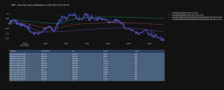
Now we will try and display our plot above the table of relevant data:
import plotly.graph_objects as go # Plotly is a great library to display interactive graphs and tables; `go` will allow us to add them on top of one-another.
from plotly.subplots import make_subplots # To have plotly elements next to each other, we'll use `make_subplots`.
# import re # If you would like to programatically change column names, you will need `re`.
import plotly
plotly.__version__
'5.8.2'
fig = make_subplots( # `fig` will be our overall figure in which we will add objects.
rows=2, cols=1, # Let's put our objects on top of each other, so 2 rows and 1 column.
shared_xaxes=True,
vertical_spacing=0.1,
specs=[[{"type": "scatter"}],
[{"type": "table"}]])
for i in fxPlotDf.columns:
fig.add_trace( # Here we're adding line traces on the graph
go.Scatter(
x=fxDf.index,
y=fxPlotDf[i],
name=i),
row=1, col=1) # Here we're indicating taht we are adding lines to a plot that is 1st (i.e.: on top) in the figure.
fig.add_trace(
go.Table( # Now we can add our table.
header=dict(
values=df.columns.to_list(),
font=dict(size=10),
align="left"),
cells=dict(
values=[df[k].tolist() for k in df.columns],
align = "left")),
row=2, col=1)
fig.update_layout(
height=800,
showlegend=True,
title_text=f'GBP= since last report publication at {df.index[-1]}', # note that `lastReportTime.strftime("%Y-%m-%dT%H:%M:%S")` and `df.index[-1]` are the same.
template = 'plotly_dark')
fig.show()
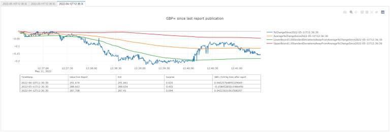
Widget
(Credit to ac24)
We can now look into incorporating our above graph in a widget that allows us to toggle between graph and data (in a table). This is a rudimentary example taken from CodeBook examples (in '__ Examples __/04. Advanced UseCases/04.01. Python Apps/EX_04_01_02__WFCH_Company_Income_Statement_Waterfall.ipynb'), but more complex ones can easily be constructed to fit your workflow.
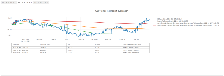
dfs['fxPlotDf'][0]
| GBP= | %ChangeSince2022-04-12T12:36:30 | Average%ChangeSince2022-04-12T12:36:30 | UpperBoundOfStandardDeviationOf%ChangeSince2022-04-12T12:36:30 | LowerBoundOfStandardDeviationOf%ChangeSince2022-04-12T12:36:30 |
|---|---|---|---|---|
| Timestamp | ||||
| 2022-04-12 12:36:31.761000+00:00 | 0.000000 | NaN | NaN | NaN |
| 2022-04-12 12:36:32.194000+00:00 | -0.003840 | 0.000000 | NaN | NaN |
| 2022-04-12 12:36:32.778000+00:00 | -0.007679 | -0.001920 | 7.952188e-04 | -0.004635 |
| 2022-04-12 12:36:33.774000+00:00 | -0.007679 | -0.003840 | -2.841911e-15 | -0.007679 |
| 2022-04-12 12:36:34.805000+00:00 | -0.007679 | -0.004800 | -1.123379e-03 | -0.008476 |
| ... | ... | ... | ... | ... |
| 2022-04-12 12:51:28.545000+00:00 | 0.076793 | 0.074129 | 1.081448e-01 | 0.040112 |
| 2022-04-12 12:51:29.553000+00:00 | 0.084472 | 0.074131 | 1.081342e-01 | 0.040127 |
1345 rows × 4 columns
%matplotlib inline
import ipywidgets as widgets
out1 = widgets.Output()
out2 = widgets.Output()
out3 = widgets.Output()
# In our example here, were are only 3 rows in `df` for which we have tick data, but we could have more and use: `outL = [widgets.Output() for i in range(len(df.dropna()))]`
tab = widgets.Tab(children=[out1, out2, out3])
for i, j in enumerate([df.index[i] for i in range(-1, -4, -1)]): # Note that instead of `enumerate(`, we could have put `zip(range(3), `.
tab.set_title(i, j)
display(tab)
# Let's use a defined function for our figure creation:
def FigureOfTableAndGraph(dfsPlotDfNo, RIC='GBP=', df=df, plotDf=dfs['fxPlotDf'], plotTemplate=None, graphHeight=800):
'''FigureOfTableAndGraph(dfsPlotDfNo, RIC='GBP=', df=df, plotDf=dfs['fxPlotDf'], plotTemplate=None, graphHeight=800) V1.0:
This python function outputs a plotly figure layout with two elements, two subplots (rows=2, cols=1); a plotly line graph above a table.
Dependencies
----------
Python library 'pandas' version 1.2.4
plotly '5.8.2' molules 'graph_objects' and 'subplots':
import plotly.graph_objects as go # Plotly is a great library to display interactive graphs and tables; `go` will allow us to add them on top of one-another.
from plotly.subplots import make_subplots # To have plotly elements next to each other, we'll use `make_subplots`.
Parameters
----------
RIC: str
Refinitiv IdentifiCation for which the line plot is made.
Default: RIC='GBP='
df: pandas dataframe
pandas dataframe containing data wished to be in the table.
Default: df=df
plotDf: list of pandas dataframe
list of pandas dataframes, each containing data wished to be graphed.
Default: plotDf=dfs['fxPlotDf']
plotTemplate: Plotly plot template
Dictates the plotly template chosen for the line graph.
Can be one of the following: "plotly", "plotly_white", "plotly_dark", "ggplot2", "seaborn", "simple_white", "none" or None.
More on templates: https://plotly.com/python/templates/
Default: plotTemplate=None
graphHeight: int
Dictates the height of the figure in which the line graph and table will be displayed.
Default: graphHeight=800
dfsPlotDfNo: int
Dictates which of the `plotDf` will be plotted.
Returns
-------
plotly fig
'''
fig = make_subplots(
rows=2, cols=1,
shared_xaxes=True,
vertical_spacing=0.1,
specs=[[{"type": "scatter"}],
[{"type": "table"}]])
for i in plotDf[dfsPlotDfNo].columns:
fig.add_trace(
go.Scatter(
x=plotDf[dfsPlotDfNo].index,
y=plotDf[dfsPlotDfNo][i],
name=i),
row=1, col=1)
fig.add_trace(
go.Table(header=dict(values=df.columns.to_list(), font=dict(size=10), align="left"),
cells=dict(values=[df[k].tolist() for k in df.columns], align = "left")),
row=2, col=1)
fig.update_layout(
height=graphHeight,
showlegend=True, template=plotTemplate,
title_text=f'{RIC} since last report publication')
return fig
with out1: # Each `out` will be a tab.
fig = FigureOfTableAndGraph(dfsPlotDfNo = -1)
fig.show()
with out2:
fig = FigureOfTableAndGraph(dfsPlotDfNo = -2)
fig.show()
with out3:
fig = FigureOfTableAndGraph(dfsPlotDfNo = -3)
fig.show()
All Together Now
# # Some imports to start with:
import pandas as pd # `pandas` is a widely-used Python library that allows us to manipulate data-frames.
import numpy as np # `numpy` is a widely-used Python library that allows us to manipulate number arrays.
import datetime # `datetime` allows us to manipulate time as it it was data points
import warnings # Some data manipulations throw warnings that polute the display we'll build; it is thus best to remove them for now; this `warnings` library will allow us to do just that.
%matplotlib inline
import ipywidgets
import ipywidgets as widgets
import plotly
import plotly.graph_objects as go # Plotly is a great library to display interactive graphs and tables; `go` will allow us to add them on top of one-another.
from plotly.subplots import make_subplots # To have plotly elements next to each other, we'll use `make_subplots`.
# import re # If you would like to programatically change column names, you will need `re`.
for i, j in zip(['pandas', 'numpy', 'ipywidgets', 'plotly'],
[pd, np, ipywidgets, plotly]):
print(i + " version " + j.__version__)
pandas version 1.3.5
numpy version 1.21.2
ipywidgets version 7.6.3
plotly version 5.8.2
def GetDSWSDataAndFalattenColumns(tickers, fields, freq, start, adjustment=0):
'''GetDSWSDataAndFalattenColumns(tickers, fields, freq, start, adjustment=0) V1.0:
One needs a LSEG Refinitiv's Datastream DSWS API(https://developers.refinitiv.com/en/api-catalog/eikon/datastream-web-service) and a working account/license.
It works by collecting DSWS data for the `tickers`, `fields`, `freq` and `start` and flattens the MultiIndex columns it usually comes out with.
Dependencies
----------
Python library 'pandas' version 1.2.4
Python library 'DatastreamDSWS' as DSWS (!pip install DatastreamDSWS), e.g.:
>>> import DatastreamDSWS as DSWS
>>> # The username and password is placed in a text file so that it may be used in this code without showing it itself.
>>> dsws_username = open("Datastream_username.txt", "r")
>>> dsws_password = open("Datastream_password.txt", "r")
>>> ds = DSWS.Datastream(username = str(dsws_username.read()), password = str(dsws_password.read()))
>>> # It is best to close the files we opened in order to make sure that we don't stop any other services/programs from accessing them if they need to.
>>> dsws_username.close()
>>> dsws_password.close()
Parameters
----------
`tickers`, `fields`, `freq` and `start`: str
For information on these function parameters, please run:
import DatastreamDSWS as DSWS
ds = DSWS.Datastream(username = "USERNAME", password = "PASSWORD"))
help(ds)
adjustment: int
I found that someties the column number was not nessesarily correct, so you can adjust it here.
Default: adjustment=0
Returns
-------
pandas dataframe
'''
df = ds.get_data(tickers=tickers, fields=fields, start=start, freq=freq)
columns = [[df.columns[i][j] for i in range(len(df.columns))]
for j in range(len(df.columns[0]) + adjustment)]
columns = [k + "_" + l for k, l in zip(columns[0], columns[1])]
df = pd.DataFrame(data=df.values, columns=columns, index=df.index)
return df
def FigureOfTableAndGraph(dfsPlotDfNo, df, plotDf, RIC='GBP=', plotTemplate=None, graphHeight=600):
'''FigureOfTableAndGraph(dfsPlotDfNo, RIC='GBP=', df=df, plotDf=dfs['fxPlotDf'], plotTemplate=None, graphHeight=800) V1.0:
This python function outputs a plotly figure layout with two elements, two subplots (rows=2, cols=1); a plotly line graph above a table.
Dependencies
----------
Python library 'pandas' version 1.2.4
plotly '5.8.2' molules 'graph_objects' and 'subplots':
import plotly.graph_objects as go # Plotly is a great library to display interactive graphs and tables; `go` will allow us to add them on top of one-another.
from plotly.subplots import make_subplots # To have plotly elements next to each other, we'll use `make_subplots`.
Parameters
----------
RIC: str
Refinitiv IdentifiCation for which the line plot is made.
Default: RIC='GBP='
df: pandas dataframe
pandas dataframe containing data wished to be in the table.
Default: df=df
plotDf: list of pandas dataframe
list of pandas dataframes, each containing data wished to be graphed.
Default: plotDf=dfs['fxPlotDf']
plotTemplate: Plotly plot template
Dictates the plotly template chosen for the line graph.
Can be one of the following: "plotly", "plotly_white", "plotly_dark", "ggplot2", "seaborn", "simple_white", "none" or None.
More on templates: https://plotly.com/python/templates/
Default: plotTemplate=None
graphHeight: int
Dictates the height of the figure in which the line graph and table will be displayed.
Default: graphHeight=800
dfsPlotDfNo: int
Dictates which of the `plotDf` will be plotted.
Returns
-------
plotly fig
'''
fig = make_subplots(
rows=2, cols=1,
shared_xaxes=True,
vertical_spacing=0.1,
specs=[[{"type": "scatter"}],
[{"type": "table"}]])
for i in plotDf[dfsPlotDfNo].columns:
fig.add_trace(
go.Scatter(
x=plotDf[dfsPlotDfNo].index,
y=plotDf[dfsPlotDfNo][i],
name=i),
row=1, col=1)
fig.add_trace(
go.Table(header=dict(values=df.dropna().loc[::-1].columns.to_list(), font=dict(size=10), align="left"),
cells=dict(values=[df.dropna().loc[::-1][k].tolist() for k in df.dropna().loc[::-1].columns], align = "left")),
row=2, col=1)
fig.update_layout(
height=graphHeight,
showlegend=True, template=plotTemplate,
title_text=f'{RIC} since last report publication')
return fig
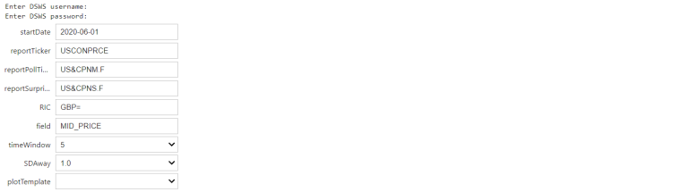
def DisplayApp(startDate='2020-06-01', reportTicker='USCONPRCE',
reportPollTicker='US&CPNM.F', reportSurpriseTicker='US&CPNS.F',
RIC="GBP=", field='MID_PRICE', timeWindow=5, SDAway=1, plotTemplate=None):
'''DisplayApp(startDate='2020-06-01', reportTicker='USCONPRCE', reportPollTicker='US&CPNM.F', reportSurpriseTicker='US&CPNS.F', RIC="GBP=", field='MID_PRICE', timeWindow=5, SDAway=1, plotTemplate=None) V1.0:
This python function outputs a plotly widget with several tabs, each showing a plotly fig with two elements: a plotly line graph above a table.
Dependencies
----------
os (native)
numpy version 1.21.2 as np
pandas version 1.2.4 as pd
plotly version 5.8.2:
import plotly.graph_objects as go # Plotly is a great library to display interactive graphs and tables; `go` will allow us to add them on top of one-another.
from plotly.subplots import make_subplots # To have plotly elements next to each other, we'll use `make_subplots`.
ipywidgets version 7.6.3:
import ipywidgets as widgets
DatastreamDSWS and instance `ds`, e.g.:
>>> import DatastreamDSWS as DSWS
>>> # The username and password is placed in a text file so that it may be used in this code without showing it itself.
>>> dsws_username = open("Datastream_username.txt", "r")
>>> dsws_password = open("Datastream_password.txt", "r")
>>> ds = DSWS.Datastream(username = str(dsws_username.read()), password = str(dsws_password.read()))
>>> # It is best to close the files we opened in order to make sure that we don't stop any other services/programs from accessing them if they need to.
>>> dsws_username.close()
>>> dsws_password.close()
refinitiv.data 1.0.0b10 as rd, e.g.:
>>> import os # This module provides a portable way of using operating system dependent functionality.
>>> os.environ["RD_LIB_CONFIG_PATH"] = "C:\\Example.DataLibrary.Python-main\\Example.DataLibrary.Python-main\\Configuration" # Here we point to the path to our configuration file.
>>> # To install the RD library, you may need to run `!pip install refinitiv-data` in Jupyter Lab/Notebook1.
>>> import refinitiv.data as rd # pip install httpx==0.21.3
>>> rd.open_session("desktop.workspace") # Send info to the Refinitiv system (i.e.: the API)
>>> # rd.open_session("desktop.workspace") # If running this code outside CodeBook. You can also try "platform.rdp"
>>> # rd.open_session("") # If running this code within CodeBook. # 'DEFAULT_CODE_BOOK_APP_KEY' is also often used in CodeBook. More on CodeBook here: https://www.refinitiv.com/content/dam/marketing/en_us/documents/fact-sheets/codebook.pdf
Parameters
----------
startDate: str
String in the form YYY-MM-DD as to when user would like data collected from.
Default: startDate='2020-06-01'
reportTicker: str
String of the numonic for the report in question in DSWS.
Default: reportTicker='USCONPRCE'
reportPollTicker: str
String of the numonic for the poll expected value for the report in question in DSWS.
Default: reportPollTicker='US&CPNM.F'
reportSurpriseTicker: str
String of the numonic for the surprise between the poll expected value and the realised value for the report in question in DSWS.
Default: reportSurpriseTicker='US&CPNS.F'
RIC: str
Refinitiv IdentifiCation for which the line plot is made.
Default: RIC='GBP='
field: str
the field for which the RIC's data will be ploted.
Default: field='MID_PRICE'
timeWindow: int
The time window, in minutes, for which tickdata is asked for, called for from the rd library and plotted. The expanding average over that window will also be plotted as well as lower and upper standard deviation bounds.
Default: timeWindow=5
SDAway: int
The standard deviation of the tick data for which the lower and upper standard deviation bounds will be plotted.
Default: SDAway=1
plotTemplate: Plotly plot template
Dictates the plotly template chosen for the line graph.
Can be one of the following: "plotly", "plotly_white", "plotly_dark", "ggplot2", "seaborn", "simple_white", "none" or None.
More on templates: https://plotly.com/python/templates/
Default: plotTemplate=None
Returns
-------
plotly fig
'''
# # Collect report data:
warnings.filterwarnings('ignore') # certain manipulations below will create warning messsages that will polute our widget, this line removes them.
reportActual = GetDSWSDataAndFalattenColumns(
tickers = reportTicker,
fields = ['X', 'TREL1', 'DREL1'],
start = startDate, freq = 'M')
reportPoll = GetDSWSDataAndFalattenColumns(
start = startDate,
tickers = reportPollTicker,
fields = "X", freq = 'M')
reportSurprise = GetDSWSDataAndFalattenColumns(
start = startDate,
tickers = reportSurpriseTicker,
fields = 'X', freq = 'M')
reportDf = pd.merge(
pd.merge(
reportActual, reportPoll, left_index=True, right_index=True),
reportSurprise, left_index=True, right_index=True).dropna()
plotDf = reportDf[[reportTicker + '_X', reportPollTicker + '_X', reportSurpriseTicker + '_X']]
plotDf.index = reportDf[reportTicker + '_DREL1']
for i in plotDf.columns:
plotDf[i] = [float(j) for j in plotDf[i].to_list()]
df = plotDf.copy()
# # Collect Tick Data:
_dfs = {'fromTime': [], 'toTime': [], 'df': [], 'prctChg': [], 'plotDf' : []} # In this dictionary, there will be a list full of all the datafames collected 7 the percent change that we're after
for i in range(len(reportDf.dropna())):
_lastReportTime = datetime.datetime.strptime(
reportDf.dropna()[reportTicker + '_DREL1'][i] + "T" + reportDf.dropna()[reportTicker + '_TREL1'][i], "%Y-%m-%dT%H:%M:%S")
_toTime = _lastReportTime + datetime.timedelta(minutes=timeWindow) # This object will be the time we're collecting tick-data until.
try:
_df = rd.content.historical_pricing.events.Definition(
universe=RIC,
fields=[field], # ['TR.BIDPRICE', 'TR.BIDPRICE.date']
start=_lastReportTime.strftime("%Y-%m-%dT%H:%M:%S"),
end=_toTime.strftime("%Y-%m-%dT%H:%M:%S")).get_data().data.df
_df.drop('EVENT_TYPE', inplace=True, axis=1) # This is a column of str's, which can mess up with the maths and plots we want to do
for i in _df.columns:
_df[i] = _df[i].astype(float) # `MID_PRICE` data is returned in str form, we would like it in float so that we can do some maths with it.
_df['%ChangeSince' + _lastReportTime.strftime("%Y-%m-%dT%H:%M:%S")] = ((
_df[field] - _df[field][0])/_df[field][0])*100
_df['Average%ChangeSince' + _lastReportTime.strftime("%Y-%m-%dT%H:%M:%S")] = [
np.average(_df['%ChangeSince' + _lastReportTime.strftime("%Y-%m-%dT%H:%M:%S")].iloc[0:i])
for i in range(len(_df))]
_dfs['fromTime'].append(_lastReportTime.strftime('%Y-%m-%dT%H:%M:%S'))
_dfs['toTime'].append(_toTime.strftime("%Y-%m-%dT%H:%M:%S"))
_dfs['df'].append(_df)
_dfs['prctChg'].append(_df['%ChangeSince' + _lastReportTime.strftime("%Y-%m-%dT%H:%M:%S")].iloc[-1])
_dfs['plotDf'].append(1)
except:
pass
np.seterr(all="ignore") # certain manipulations below will create warning messsages that will polute our widget, this line removes them.
for i in range(len(_dfs['df'])):
_dfs['df'][i][f'StandardDeviation{SDAway}Of%ChangeSince' + _dfs['fromTime'][i]] = [
_dfs['df'][i]['%ChangeSince' + _dfs['fromTime'][i]].iloc[0:j].std() * SDAway
for j in range(len(_dfs['df'][i]))]
_dfs['df'][i][f'UpperBound{SDAway}StandardDeviationsAwayFromAverage%ChangeSince' + _dfs['fromTime'][i]] = [
_dfs['df'][i]['Average%ChangeSince' + _dfs['fromTime'][i]].iloc[j] +
_dfs['df'][i][f'StandardDeviation{SDAway}Of%ChangeSince' + _dfs['fromTime'][i]].iloc[j]
for j in range(len(_dfs['df'][i]))]
_dfs['df'][i][f'LowerBound{SDAway}StandardDeviationsAwayFromAverage%ChangeSince' + _dfs['fromTime'][i]] = [
_dfs['df'][i]['Average%ChangeSince' + _dfs['fromTime'][i]].iloc[j] -
_dfs['df'][i][f'StandardDeviation{SDAway}Of%ChangeSince' + _dfs['fromTime'][i]].iloc[j]
for j in range(len(_dfs['df'][i]))]
_dfs['plotDf'][i] = _dfs['df'][i][[
'%ChangeSince' + _dfs['fromTime'][i],
'Average%ChangeSince' + _dfs['fromTime'][i],
f'LowerBound{SDAway}StandardDeviationsAwayFromAverage%ChangeSince' + _dfs['fromTime'][i],
f'UpperBound{SDAway}StandardDeviationsAwayFromAverage%ChangeSince' + _dfs['fromTime'][i]]]
# # If you would like to rename columns in a programatic way, you can import `re` and use the lines below:
# _dfs['fxPlotDf'][i].columns = [
# re.sub(r"(\w)([A-Z])", r"\1 \2", j)
# for j in _dfs['fxPlotDf'][i].columns]
# # Proccess data:
df.index=[reportDf[reportTicker + '_DREL1'] + 'T' + reportDf[reportTicker + '_TREL1']]
prctChg = [np.nan for i in range(len(df) - len(_dfs['prctChg']))]
for i in _dfs['prctChg']: prctChg.append(i)
df[RIC + ' PrctChg ' + str(timeWindow) + 'min after report'] = prctChg
df.rename(columns={reportTicker + '_X':'Value from Report',
reportPollTicker + '_X' :'Poll',
reportSurpriseTicker + '_X' :'Surprise'},
inplace = True)
df.insert(0, 'TimeStamp', df.index.values)
# # Create widget and plots:
outL = [widgets.Output() for i in range(len(df.dropna()))]
tab = widgets.Tab(children=outL)
for i, j in enumerate([df.index[k] for k in range(-1, (len(outL)*-1)-1, -1)]):
tab.set_title(i, j)
display(tab)
for i, out in enumerate(outL):
with out:
fig = FigureOfTableAndGraph(
dfsPlotDfNo=-1*i, df=df, plotDf=_dfs['plotDf'], RIC=RIC, plotTemplate=plotTemplate)
fig.show()
Kudos to Kimberly Fessel
# # Authentification to LSG Refinitiv's Datastream Service:
import DatastreamDSWS as DSWS # We can use our Refinitiv's Datastream Web Socket (DSWS) API keys that allows us to be identified by Refinitiv's back-end services and enables us to request (and fetch) data
import getpass as gp # This library will allow users to entre their passwords without showing it to anyone watching.
dsws_username = input("Enter DSWS username:")
dsws_password = gp.getpass("Enter DSWS password:")
if dsws_username == "" and dsws_password == "": # Users might have their credentials in .txt files along side their code, in which case we code bellow so that if the username and password are left empty, we automatically look for and use those txt files.
dsws_username = open("Datastream_username.txt", "r")
dsws_password = open("Datastream_password.txt", "r")
ds = DSWS.Datastream(username = str(dsws_username.read()), password = str(dsws_password.read()))
dsws_username.close()
dsws_password.close()
else:
ds = DSWS.Datastream(username = dsws_username, password = dsws_password)
# # Let's use the Refinitiv Data Library for Python (RD)
import refinitiv.data as rd # pip install httpx==0.21.3
try: # To use the RD library in Codebook, we don't need any user credentials
rd.open_session("")
connectionTest = rd.content.historical_pricing.events.Definition(
'VOD.L').get_data().data.df # `connectionTest` is just a test value to see if we're connected to rd.
except: # To use the RD library outside of codebook, we need to ask user where the config file is:
import os # This module provides a portable way of using operating system dependent functionality.
creds = input("Enter the path to your 'refinitiv-data.config.json' file and the session wished (e.g.1: C:\\Example.DataLibrary.Python-main\\Configuration,desktop.workspace) (e.g.2: C:\\Con,platform.rdp): ")
os.environ["RD_LIB_CONFIG_PATH"] = creds.split(",")[0] # Here we point to the path to our configuration file.
rd.open_session(creds.split(",")[1]) # Send info to the Refinitiv system (i.e.: the API)
try:
connectionTest = rd.content.historical_pricing.events.Definition(
'VOD.L').get_data().data.df # `connectionTest` is just a test value to see if we're connected to rd.
except:
print("Connection to RD could not be established")
# # Now let's start up the Widget:
widgets.interact( # NonFarmPayRoll: reportTicker = 'USPENOACO', reportPollTicker = 'US&ADPM.O', reportSurpriseTicker = 'US&ADPS.O'
DisplayApp,
timeWindow=[i for i in range(1, 61)],
SDAway=[i/10 for i in range(1, 31)],
plotTemplate=['ggplot2', 'seaborn', 'simple_white', 'plotly',
'plotly_white', 'plotly_dark', 'presentation',
'xgridoff', 'ygridoff', 'gridon', 'none']); # The `;` is there to stop the widget message from showing up.
References
You can find more detail regarding the Datastream API and related technologies for this notebook from the following resources:
- Refinitiv Data API page on the LSEG Refinitiv Developer Community web site.
- Datastream DSWS Python Tutorial Series/Article 'Estimating Monthly GDP via the Expenditure Approach and the Holt Winters Model'.
For any question related to this example or Datastream's API (DSWS), please use the Developers Community Q&A Forum.