
ABOUT THE MODEL
The cmdty_seasonality.ipynb is a python model that uses Eikon Data API for seasonality charting of commodity futures. This file is designed to be imported as a module into other jupyter notebooks using the ipynb python library and used by calling the main calculation function:
cmdty_seasonality.get_data(ric, lookback_years, month, rebase)
The input descriptions are given below:
| Parameter | Description | Possible argument |
| ric | A futures contract RIC. NOTE: The function does not support continuous futures RICs. | string, e.g. LGOK0 |
| lookback_years | The number of expired contracts that the method will loop up. Default value = 5. | int |
| month | The month of the year, which will be plotted on the chart. Default value = current month. | int |
| rebase | Performs rebasing of the timeseries to 0. Default value = False | bool |
The function returns a plotly chart as well as a pandas dataframe with the historical data.
IMPORTING DEPENDENCIES
The model uses Eikon Data API as a data source, and will be performing date manipulations, therefore we will reference the following libraries:
import eikon as ek
import numpy as np
import calendar
import cufflinks as cf
import pandas as pd
from pandas.tseries.offsets import BMonthEnd
from datetime import datetime
cf.go_offline()
app_key = 'YOUR_APP_KEY'
ek.set_app_key(app_key)
This script contains several auxilary functions, which will be covered in the next section, as we walk through main method get_data().
RUNNING THE SCRIPT
Let's look at the step-by-step code execution for getting the seasonality data on a crude oil futures contract. Let's define our input parameters as follows:
ric = 'LCOK0'
lookback_years = 10
month = 3
rebase = True
df = get_data(ric, lookback_years, month, rebase)
The RIC LCOK0 stands for a Brent Crude Futures [LCO] + delivery month [K] (May) + delivery year [0] (2020) - we will be using this structure to create the identifiers for the expired contracts from previous years. Since lookback_years is 10 and month is 3, we will be comparing the timeseries for the May futures contracts within the 3rd month (i.e. March) during the past 10 years. And we will be looking at rebasing the chart to capture the percent change for every period - hence we set rebase to True. Now let's start the calculation by plugging these into get_data().
When the function is called, it will construct a list of RICs for futures contracts (including the current one) and retrieve the timeseries for the given month in previous years:
def get_data(ric, lookback_years = 5, month = current_month(), rebase = False):
if 'c' in ric:
return 'Please enter a futures delivery month contract code (e.g. LCOK0).'
frames = gen_contracts(ric, lookback_years, month)
hist = get_timeseries_seq(frames)
. . .
The first auxilary function gen_contracts() creates a list of lists, that stores the futures RICs, start and end dates for the timeseries:
def gen_contracts(r, d, m):
xd, err = ek.get_data(r, 'EXPIR_DATE')
xd = xd['EXPIR_DATE'][0]
xd = xd.split('-')
y = xd[0]
_m = int(xd[1]) if m is None else m
_y = int(y)
_x = []
x = []
root = contract_data(r)
while d >= 0:
if d == 0:
_x = ('{}{}'.format(root, str(_y - d)[-1:]))
_ed = eom(_y-d, _m)
else:
dec = str(_y - d)[-2:][0]
_x = '{}{}^{}'.format(root, str(_y - d)[-1], dec)
_ed = eom(_y-d, _m)
_sd = som(_y-d, _m)
x.append([_x, _sd, _ed])
d -= 1
return x
The way this function works is that we first get the expiration date of the input futures contract from the field EXPIR_DATE with Eikon Data API. For example, LCOK0 will expire on 2020-03-31. This string value is then parsed to form a list with the year, month and date of expiration. We then combine the root of the contract ticker (i.e. LCOK) with a suffix, that indicated the year and decade of expiration. The RIC structure for expired future contracts follows this logic:
[futures ticker] + [month of delivery code] + [year of delivery] + [ ^ ] + [decade of delivery],
where decade of delivery is given as a single digit: 2020s = 2, 2010s = 1, 2000s = 0, 1990s = 9, etc. In this example, the returned list of lists looks as follows:
In [2]:
gen_contracts('LCOK0', 10, 3)
Out [2]:
[['LCOK0^1', '2010-03-01', '2010-03-31'],
['LCOK1^1', '2011-03-01', '2011-03-31'],
['LCOK2^1', '2012-03-01', '2012-03-30'],
['LCOK3^1', '2013-03-01', '2013-03-29'],
['LCOK4^1', '2014-03-01', '2014-03-31'],
['LCOK5^1', '2015-03-01', '2015-03-31'],
['LCOK6^1', '2016-03-01', '2016-03-31'],
['LCOK7^1', '2017-03-01', '2017-03-31'],
['LCOK8^1', '2018-03-01', '2018-03-30'],
['LCOK9^1', '2019-03-01', '2019-03-29'],
['LCOK0', '2020-03-01', '2020-03-31']]
The root of the contact ticker is parsed from the input RIC, by the auxilary function contract_data():
def contract_data(r):
k = list(r)
root = ''.join(k[:-1])
return root
As we can see, it simply trims the last digit denoting the year of delivery for the futures RIC. In our example, the root will be LCOK.
The start and end date of the month are calculated using the auxilary functions som() and eom():
def last_workday(d):
last = BMonthEnd()
return last.rollforward(d)
def eom(y, m):
ed = last_workday(datetime(year = int(y), month=m, day=1)).strftime('%Y-%m-%d')
return ed
def som(y, m):
sd = datetime(year = int(y), month=m, day=1).strftime('%Y-%m-%d')
return sd
The eom() function uses the BMonthEnd method to get the last business day of the given month to avoid getting data for the unnecessary weekends.
Now that the list of contract RICs and dates has been created, we move on to retrieving the historical prices for these instruments with get_timeseries_seq(). This function cycles through the list of lists displayed earlier and uses the get_timeseries() method of Eikon Data API to retrieve the history and store result in a dictionary with a structure like: {RIC : time_series}.
def get_timeseries_seq(l):
d = {}
for i in l:
d[i[0]] = ek.get_timeseries(i[0], 'CLOSE', start_date=i[1], end_date=i[2], interval='daily')
return d
At this point we have all the data we need, and the remining portion of get_data() focuses on aligning the dates so that we have a direct comparison between the contracts ignoring the year values:
. . .
for k in hist.keys():
_idx = []
for i in range(len(hist[k])):
_idx.append(list(hist[k].index)[i].strftime('%b-%d'))
hist[k]['Dates'] = _idx
seasonal_df = pd.DataFrame(columns = ['Dates'])
for k in hist.keys():
seasonal_df = pd.merge(seasonal_df, hist[k], on='Dates', how = 'outer')
. . .
The first loop re-formats each dataframe index by dropping the year, whereas the second loop merges all dataframes by mapping the historical values to the same index intries. The last snippet backfills any data gaps in the aggregated dataframe and adds the necessary labels to the columns, so that the each series would be named accordingly on the plotly chart:
. . .
seasonal_df = seasonal_df.sort_values(by='Dates')
seasonal_df = seasonal_df.fillna(method='backfill')
seasonal_df = seasonal_df.reset_index(drop = True)
seasonal_df.index = seasonal_df['Dates']
seasonal_df = seasonal_df.drop(columns='Dates')
seasonal_df.columns = list(hist.keys())
title = 'Seasonality chart'
ytitle = 'Price'
if rebase:
seasonal_df = pd.DataFrame((np.log(seasonal_df)-np.log(seasonal_df.iloc[0])))*100
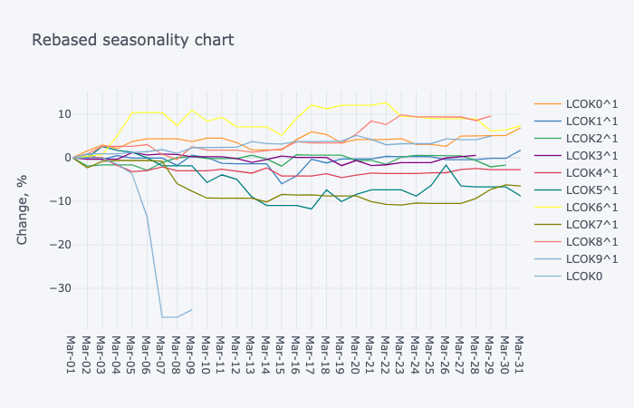
title = 'Rebased seasonality chart'
ytitle = 'Change, %'
seasonal_df.iplot(title=title, yTitle = ytitle)
return seasonal_df
Since we have chosen to rebase the values and capture the percent change of each series, the script gets the log returns in the last if-statement, alternatively it would be ignored. The output is stored in a pandas dataframe, and we build a plotly chart using cufflinks, which will look similar to the ne below (NOTE: the sharp decline in LCOK0 vs previous years caused by the failed OPEC agreement to reduce oil production in March 2020):