


Introduction
There has been a growing interest for direct data access, management and analytical tools in the commodity trading space. Refinitiv Data Management Solutions (RDMS) is designed to serve the purpose, helping clients to ingest and standardize data and perform more advanced data analysis efficiently in their daily work. As part of the RDMS case studies series, we have joined with Refinitiv’s North American Natural Gas Research team to exhibit how the RDMS platform can be used effectively to perform insightful data analysis in the commodities trading field, specifically for the natural gas market. As a Refinitiv Eikon commodity and RDMS suites subscriber, one can access a plethora of Refinitiv’s comprehensive datasets backed by the best-performing models. In particular, Refinitiv’s North American Gas team has produced excellent models, placing us among the top forecasters in the U.S. for Natural Gas storage and pricing. The goal of this project was to effectively combine the automated and real-time run output from various NA Gas models (which are available in PointConnect Gas Packages) with supplementary data provided by RDMS as well as any 3rd party data we deem fit.
In this case study, RDMS allows us to retrieve the regional power generation data by fuel and combine it with other input price variables, most notably regional gas cash prices from Natural Gas Intelligence (NGI). Regional gas price has traditionally been an important economic factor for power generators with dual fuel availability. Depending on the prices of gas and coal, operators generally have the flexibility to make the decision in a relatively short manner to switch between gas-fired and coal-fired generation to meet forecast demand. Given the easy API data access and completeness of the datasets on RDMS platform, in our discussions we realized this would be a great opportunity for us to review our regional Coal-to-Gas switching forecast. A side-by-side comparison against our current synthetic demand estimates would provide additional values for NA gas forecast and potentially help enhance our model performance and recalibration process. For the purpose of this project, we each chose a region to exhibit, these selected regions were the Electric Reliability Council of Texas (ERCOT), South-West Power Pool (SWPP), PJM Interconnection (PJM), MidContinent Independent System Operator (MISO). These organizations were chosen as they are the largest consumers of gas and coal.
Getting started
Both RDMS and Eikon Data APIs require the use of app keys at runtime. Please refer to the Quick Start guides for RDMS and for Eikon Data APIs for instruction on how to set up and use these app keys.
Since regional prices are seasonal and communally affected by movement in national prices (the Henry Hub reference price) our early analyses were skewed by noise from regional prices that did not logically make sense for the region we were looking at (i.e., some regressions for the MidContinent ISO showed abnormally large dependence on minor prices located in Appalachia and Florida). To adjust for this issue we placed prices into regions and excluded those that would not be expected to affect demand from the regions’ analyses. The RICs were gathered from Eikon and placed in a CSV file named NGI_PriceRegions.csv. We then added the state where the prices are located and put into regions.
ngi_RIC = pd.read_csv('NGI_PriceRegions.csv',index_col=0)
Retrieving and organizing data
In this project we used two methods for retrieving data. For pricing data we developed a function named getRICData. This function is implemented in the C2GTest.py module, which you can find in the source code repository for this article on GitHub. This function takes RIC names and start and end date as inputs, and uses the Eikon Data APIs to retrieve timeseries of close prices, which it then converts this into a matrix. Since it uses Eikon Data APIs, the function requires that Eikon or Refinitiv Workspace are running on the same machine where the function is being executed.
def getRICData(RICs,startdate,enddate):
curve_data = list(map(lambda x: ek.get_timeseries(x,'Close',startdate,enddate,'daily'),RICs))
for idx, sub_df in enumerate(curve_data):
sub_df.columns = [RICs[idx]]
return pd.concat(curve_data, axis=1)
The other method is used to retrieve curves from RDMS. We developed 6 functions, which can be seen in the rdms_gas.py module available from the source code repository for this article on GitHub. The module includes 6 functions. getForecast, getLatestForecast and getTimeSeries are used to retrieve data from a single curve for forecasts from a specific date, latest forecast, and timeseries respectively. getForecastMatrix, getLatestForecastMatrix and getTimeSeriesMatrix functions take multiple curve IDs as input, call one of the former 3 functions and transform the output into a matrix. These three options function similarly, they just require slightly different inputs. The most important package for these functions is requests, which is how the data is fetched from RDMS through a url. To retrieve data from RDMS endpoint we need to create HTTP request header with the app key..
headers = {'Authorization' : rdms_demo_app_key}
Now we can send a request to fetch regional power generation forecast by fuel curve using curve ID and forecast date as inputs.
res = requests.get('https://demo.rdms.refinitiv.com/api/v1/CurveValues/Forecast/'+
curveid + '/0/' + ForecastDate,headers=headers, verify=True)
The rest is a matter of how you want to present the data. For our purposes we preferred a pandas dataframe.
curve_data = pd.DataFrame.from_dict(res.json())
Assign prices to regions and run the analysis
Once we had the list of reasonable prices, we created dictionaries to match each organization with the RIC codes and names of the possible prices. In our early analyses we found prices to be one of the strongest predictors of coal-to-gas switching, however the Henry Hub gas futures prompt month (RIC = NGc1) and McCloskey Coal PRB futures prompt month (RIC = CQPR8C1) prices were not as great for daily changes, so a local cash price would be necessary. We created four different runs for each region:
1. singleprice = CQPR8C1 & NGc1 + a single regional price
2. singleprice_NGc1 = CQPR8C1 + NGc1 or a single regional price
3. doubleprice = CQPR8C1 & NGc1 + two regional price
4. doubleprice_NGc1 = CQPR8C1 + NGc1 and a single price or two regional price
We also created exclusion_dates, which ignore the results during the February 2021 blackout in Texas, since prices were skewed in that time.
The regional analyses were performed using a function we created in our C2GTest library called RegionalC2GTest. This function was based on our early analyses, where we just sought to find the effect of various energy sources on the Gas/Coal ratio. RegionalC2GTest receives 9 inputs:
1. Region name
2. Fixed prices
3. Spot RICs (we used the regional price RICs from before, and add NGc1 when it is not a fixed price)
4. The amount of Spot RICs being used (in this case we only do 1 or 2)
5. The name of the spot RICs
6. How many days the RICs must be shifted (the RICS are day-ahead prices)
7. An option to retrieve the ISO generation data in the function or use a previously retrieved dataset
8. An option to retrieve the price data in the function or use a previously retrieved dataset
9. A dataset for dates to be excluded from the analysis (i.e. the Texas Blackout)
We tested each region with a linear regression analysis for each price combination. These combinations were put into separate dictionaries, where we could access and review which options returned the best results for every region.
ric = dict()
names = dict()
ric['MISO'] = list(ngi_RIC.index[ngi_RIC['REGION'].str.match('Mid-Continent|MidWest|LA')])
names['MISO'] = list(ngi_RIC.NAME[ngi_RIC['REGION'].str.match('Mid-Continent|MidWest|LA')])
ric['ERCO'] = list(ngi_RIC.index[ngi_RIC['REGION'].str.match('TX|LA')])
names['ERCO'] = list(ngi_RIC.NAME[ngi_RIC['REGION'].str.match('TX|LA')])
ric['SWPP'] = list(ngi_RIC.index[ngi_RIC['REGION'].str.match('TX|LA|Mid-Continent')])
names['SWPP'] = list(ngi_RIC.NAME[ngi_RIC['REGION'].str.match('TX|LA|Mid-Continent')])
ric['PJM'] = list(ngi_RIC.index[ngi_RIC['REGION'].str.match('Appalachia|MidWest')])
names['PJM'] = list(ngi_RIC.NAME[ngi_RIC['REGION'].str.match('Appalachia|MidWest')])
singleprice = dict()
singleprice_NGc1 = dict()
doubleprice = dict()
doubleprice_NGc1 = dict()
regions = ['MISO','SWPP','ERCO','PJM']
# exclude the Texas Blackout period
exclusion_dates = pd.date_range(start='02/10/2021', end='03/01/2021', freq='D')
for i in regions:
singleprice[i],isodata,price_df = C2GTest.RegionalC2GTest(i,['CQPR8C1','NGc1'], ric[i],1,names[i], 0, 0, 0,exclusion_dates)
doubleprice[i],_,_ = C2GTest.RegionalC2GTest(i,['CQPR8C1','NGc1'], ric[i],2,names[i], 0,isodata,price_df,exclusion_dates)
singleprice_NGc1[i],_,_ = C2GTest.RegionalC2GTest(i,['CQPR8C1'],['NGc1']+ric[i],1,['NGc1']+names[i],0,isodata,price_df,exclusion_dates)
doubleprice_NGc1[i],_,_ = C2GTest.RegionalC2GTest(i,['CQPR8C1'],['NGc1']+ric[i],2,['NGc1']+names[i],0,isodata,price_df,exclusion_dates)
Prepare output
While reviewing the results, we noticed that the regression with 2 prices where NGc1 is not a fixed variable option returned the strongest R-Squared values. To analyze which specific prices worked best, we limited our choices to the top 10% of R-Squared values in the dictionary and plotted the prices that appeared most frequently. Each of the regions’ strongest performers were placed in the output dictionary.
output = dict()
for x in regions:
sublist = doubleprice_NGc1[x]
sublist = sublist[sublist['Rsq']>sublist['Rsq'].quantile(q=0.9)]
p = [[i,j] for i, j in sublist.index]
sublist2 = list(itertools.chain(*p))
df = pd.DataFrame.from_dict(collections.Counter(sublist2), orient='index', columns = ['Freq'])
output[x] = df.sort_values(by = ['Freq'])
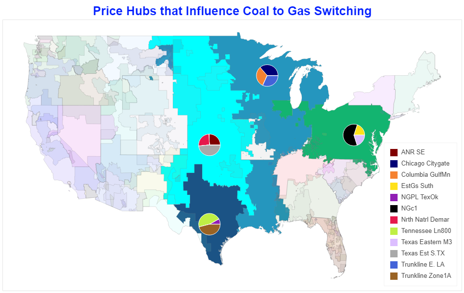
Plotting pie charts on the map
To visualize which plants have the most influence over the ratio of coal to gas on the power grid, we decided to plot the top 3 influencers for each region as a pie chart on the map of Regional Transmission Organizations. We experimented with several charting libraries and found bokeh library to be the easiest to use while also producing the best quality of map image. We used geopandas to load the map from a shape file and transform it to GeoJSON. To add the pie charts we used the Wedge class from bokeh.models module. For clarity we also added the legend to the chart and tolltips over the pie charts' wedges.
from math import pi
import geopandas as gpd
import bokeh
from bokeh.plotting import figure
from bokeh.transform import cumsum
from bokeh.io import output_notebook, show
output_notebook(hide_banner=True)
gdf = gpd.read_file('ISOMap')
geosource = bokeh.models.GeoJSONDataSource(geojson = gdf.to_json())
p = figure(title = 'Price Hubs that Influence Coal to Gas Switching',
plot_height = 600 ,
plot_width = 950,
toolbar_location = None)
p.xgrid.grid_line_color = None
p.ygrid.grid_line_color = None
p.axis.visible = False
p.title.align = "center"
p.title.text_color = "#001EFF"
p.title.text_font_size = "25px"
# Add patch renderer to figure.
chart_regions = p.patches('xs','ys', source = geosource,
fill_color = 'color',
line_color = 'gray',
line_width = 0.25,
fill_alpha = 'fill_alpha')
# Add pie charts
pie_coordinates = {'MISO': [45, -91], 'SWPP': [38, -99], 'ERCO': [30, -99], 'PJM': [39, -79]}
pie_colors = ['#800000','#000075','#F58231','#FFE119','#911EB4','#000000',
'#E6194B','#BFEF45','#DCBEFF','#A9A9A9','#4363D8','#9A6324']
pie_chart_data = dict()
for x in regions:
pie_chart_data[x] = output[x].tail(3)['Freq']
pie_chart_data = pd.DataFrame(pie_chart_data)
pie_chart_data.fillna(0, inplace = True)
pie_chart_data['Color'] = pie_colors[:len(pie_chart_data.index)]
for w in pie_coordinates.keys():
pie_chart_data[f'Angle_{w}'] = pie_chart_data[w]/pie_chart_data[w].sum() * 2*pi
renderlist = []
pie_chart_data_source = bokeh.models.sources.ColumnDataSource(pie_chart_data)
for w in pie_coordinates.keys():
lat, lon = (pie_coordinates[w][0], pie_coordinates[w][1])
r = p.wedge(x=lon, y=lat, radius=1.5, alpha=1,
start_angle=cumsum(f'Angle_{w}', include_zero=True),
end_angle=cumsum(f'Angle_{w}'),
line_color='white', fill_color='Color',
source=pie_chart_data_source)
renderlist.append(r)
p.add_tools(bokeh.models.HoverTool(tooltips = [('Price Hub', '@index'),('Region', w)], renderers=[r]))
legend = bokeh.models.Legend(items=[bokeh.models.LegendItem(label=dict(field='index'),renderers=renderlist)],
location='bottom_right')
p.add_layout(legend)
show(p)
Regional analyses
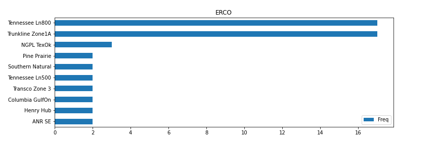
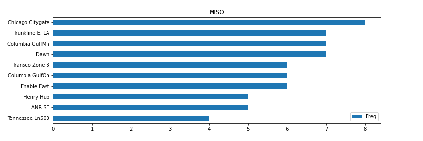
To create a regional analysis, we plot each region’s top prices separately. Once again, we sort the top prices by how often they appear in the top R-squared values for each region’s linear regressions. The top R-squared values do not vary much, which is why we go with the frequency of appearance here. This also means that slight changes (for example running this a few days later) can cause shifts in the frequencies. We noticed that this affected PJM and MISO mostly, as the prices with the top frequencies ranged from 5-7 during various runs in different days. SWPP and ERCOT showed more consistent findings.
for x in regions:
output[x].tail(10).plot.barh(figsize=(12,4),title=x)
South-West Power Pool (SWPP)
During the first 10 months of 2021, coal made up the largest share of SWPP generation, as coal plants accounted for 36.8% of all power usage in SWPP, while wind produced 32.6% of power, and natural gas produced 20.8%. SWPP is also the least populous of the four regions studied, and has the smallest daily usage, averaging around 31 GW. Thus, while coal plants are common enough that coal-to-gas switching still has a large effect on gas demand, the region is mainly a price-taker, as larger demand and supply shifts in adjacent regions produce more volatile price swings. We can see this reflected in the analysis, where only one of the nine most significant Hubs for SWPP coal-to-gas switching (Northern Natural Demarcation) is located within the boundaries of SWPP itself. Texas Eastern South Texas reflects prices in the producing region of the Eagle Ford shale, with links to important consuming areas in the Northeast and Midwest Another important point, ANR in Southern Louisiana, has a highly significant relationship to switching, as it links the volatility of Henry Hub to both SWPP and the larger consuming region of the Great Lakes. The volatility in these adjacent regions affects decisions on whether to ramp up gas-to-power production in the Great Plains states of SWPP.

PJM Interconnection (PJM)
PJM Interconnection coordinates nearly 1,400 generators in all or parts of 13 populous states in Mid-Atlantic area. Among the 180 GW total installed capacity as of year-end 2020, coal units still represent 28% of the market share (53 GW) while natural gas (78 GW) is the primary fuel for 42% of the generating capacity. This compares to roughly 68 GW of coal and 48 GW of gas capacity installed by year-end 2010. The region is conveniently sitting on top of the Appalachian Basin, home to the prolific gas and coal producing fields. Since 2010, Appalachian gas production has grown from zero to nearly 35 Bcf/d this year, eating away coal market share through permanent or economic fuel switching along the way. In 2020, the region still produced 20% of total US coal and roughly one third of dry gas supply. Having access to one of the lowest-cost fuel resources in the US, coal-to-gas switching has been very volatile and sensitive to the gas price changes in the area.
Especially considering PJM is serving nearly 65 million population, seasonal swings of the regional gas demand — stronger direct gas space heating requirements in winter vs electric gas-fired power generation loads in summer — and the resultant gas price seasonal movements ultimately lead to symbolic characteristics of the fuel switching dynamics in the region. The national benchmark NGc1 made it to the top 3 since the prompt Henry Hub trading reflects the overall anticipation of forward market tightness. Among all the pricing hubs we examine, Texas Eastern M-3 and Eastern Gas South best represent the regional seasonality and supply dynamics. Both price hubs are located relatively closer to the gas producing field. Eastern Gas South appears to be linked to the upstream Appalachian supply while Texas Eastern pipeline further extends north and delivers gas to the dense population areas in New Jersey and New York.

Electric Reliability Council of Texas (ERCOT)
ERCOT power generation stack is predominantly driven by natural gas, contributing on average 45% in 2020 and 42% (January - October) in 2021. Other important sources of energy available to generate power are from wind and coal. They accounted for 24% and 19% respectively to the stack in 2021.
In 2021, coal generation saw some growth at the very beginning of the year, up 6 percent in January compared to last year. The growth is evident again in June and July, up on average 4 percent. Meanwhile, gas generation dropped around 7% compared to last year.
Given the gas prices have run-up over the past months. We ran an analysis to help us pinpoint a particular hub that impacts gas and coal generation. Our analysis shows that Tennessee LN800 and Trunkline Zone 1A pricing points have a significant impact on coal/gas switching in ERCOT region. Other hubs such as Southern Natural and Henry Hub also show some significancy to fuel switching in the region but not to the same degree as Tennessee LN800 and Trunkline Zone 1A.
MidContinent Independent System Operator (MISO)
MISO is one of the largest regions in the country, stretching from Minnesota and parts of North Dakota as far south as Louisiana, Mississippi and eastern Texas. As such, MISO is the second largest consumer, its total generation is just under PJM’s as it averaged 70.8 GWh/d in 2021. From 2018-2020, nearly 45% of the total generation was from Coal; this has dropped slightly to 44.6% in 2021, while Gas has been used for approximately 26% of the total generation in 2021. Nuclear generation has seen the largest drop in the region, going from about 16.6% of the total generation in 2018-2020 to 15.4% in 2021. Wind on the other hand has seen the largest expansion, increasing from 10% of total generation to 12.2% in 2021.
We originally believed the best regional price would be Chicago Citygate and Dawn, as they are two of the largest hubs in the region. Both of these appeared among the top contributors for the prices in the top 10% of R-squared values, in our most recent run, however this wasn’t always the case. The other prices to appear most frequently were Columbia GulfMn and Trunkline E. LA. That being said, none of these are clear winners, and with the frequencies appearing in a smaller range compared to some other regions, they could once again shift in another run. If we were to use the cash prices to estimate the Coal to Gas ratio in the future, we would likely have to run the regression more frequently to keep up with the changing prices.
Complete source code for this article can be downloaded from Github
https://github.com/Refinitiv-API-Samples/Article.RDMS.Python.CoalToGasSwitching