ACADEMIC ARTICLE SERIES: ECONOMICS AND FINANCE INVESTIGATION:
ARMA Modelling with Arbitrary/Non-Consecutive Lags and Exogenous Variables in Python using Sympy: From Matrix Mathematics and Statistics to Parallel Computing: Part 1
Author:

This article constructs a Python function allowing anyone to discern all Maximum Likelihood Estimates of any ARMA(p,q) model using matrices, using the Python library 'Sympy'. We go through the fundamentals of ARMA models, the Log-Likelihood estimation method, matrix constructions in Sympy, and then put it all together to build our generalised model. In this 1st Part/Draft, we lay the foundations needed before continuing and make one function to encapsulate any ARMA model, with or without arbitrary lags.
Twitch Python Finance Webinar
ARMA models
An AutoRegressive Moving Average model of order $p$ and $q$ (ARMA($p,q$)) represents $y_t$ in terms of $p$ of its own lags and $q$ lags of a white noise process such that:
$$\begin{align} y_t &= c + \phi_1 y_{t-1} + \phi_2 y_{t-2} + ... + \phi_p y_{t-p} + \epsilon_t + \psi_1 \epsilon_{t-1} + \psi_2 \epsilon_{t-2} + ... + \psi_q \epsilon_{t-q} \\ y_t &= c + \left( \sum_{i=1}^{p}\phi_i y_{t-i} \right)+ \epsilon_t + \left( \sum_{j=1}^{q} \psi_j \epsilon_{t-j} \right) \\ y_t - \left( \sum_{i=1}^{p}\phi_i y_{t-i} \right) &= c + \epsilon_t + \sum_{j=1}^{q} \psi_j \epsilon_{t-j} \\ y_t - \phi_1 y_{t-1} - \phi_2 y_{t-2} - ... - \phi_p y_{t-p} &= c + \epsilon_t + \psi_1 \epsilon_{t-1} + \psi_2 \epsilon_{t-2} + ... + \psi_q \epsilon_{t-q} \\ y_t \left( 1 - \phi_1 L^1 - \phi_2 L^2 - ... - \phi_p L^{p} \right) &= c + \epsilon_t \left( 1 + \psi_1 L^1 + \psi_2 L^2 + ... + \psi_q L^{q} \right) \\ \label{eq:ARMApq} \tag{1} y_t \left( 1 - \sum_{i=1}^{p}\phi_i L^{i} \right) &= c + \epsilon_t \left( 1 + \sum_{j=1}^{q} \psi_j L^{j} \right) \end{align}$$where $L$ is the Lag opperator such that $x_t L^i = x_{t-i} $ $ \forall $ $ x, t, i \in \mathbb{R}$.
It is important to note that due to the fact that we use $p$ autoregressive and $q$ moving average componants, we use $p$ lags of our dependent variable - $y$ - and $q$ lags of our error term - $\epsilon$. This means that the first forecast produced by an ARMA($p,q$) model must use at least $max(p,q)$ lags and we thus loose these observations from our observation data-set.
$\textbf{Example:}$ Let $p = 2$ and $q = 3$, then
$$\begin{align} y_t &= c + \left( \sum_{i=1}^{2}\phi_i y_{t-i} \right)+ \epsilon_t + \left( \sum_{j=1}^{3} \psi_j \epsilon_{t-j} \right) \\ y_t - \left( \sum_{i=1}^{2}\phi_i y_{t-i} \right) &= c + \epsilon_t + \sum_{j=1}^{3} \psi_j \epsilon_{t-j} \\ y_t - \phi_1 y_{t-1} - \phi_2 y_{t-2} &= c + \epsilon_t + \psi_1 \epsilon_{t-1} + \psi_2 \epsilon_{t-2} + \psi_q \epsilon_{t-3} \\ y_t \left( 1 - \phi_1 L^1 - \phi_2 L^2 \right) &= c + \epsilon_t \left( 1 + \psi_1 L^1 + \psi_2 L^2 \psi_q L^{3} \right) \\ y_t \left( 1 - \sum_{i=1}^{2}\phi_i L^{i} \right) &= c + \epsilon_t \left( 1 - \sum_{j=1}^{3} \psi_j L^{j} \right) \end{align}$$
ARMA models' Stationarity
Now we can see that \eqref{eq:ARMApq} can be re-written such that
$$\begin{align} y_t \left( 1 - \sum_{i=1}^{p}\phi_i L^{i} \right) &= c + \epsilon_t \left( 1 + \sum_{j=1}^{q} \psi_j L^{j} \right) \\ y_t \Phi_p(L) &= c + \epsilon_t \Psi_q(L) \end{align}$$where the AR (AutoRegressive) component of our model is encapsulated in $\Phi_p(z) \equiv (1 - \sum_{i=1}^{p}\phi_i z^{i})$ and the MA (Moving Average)'s in $\Psi_q(z) \equiv (1 + \sum_{j=1}^{q} \psi_j z^{j})$ $\forall p,q,z \in \mathbb{R}$. From there, we can see that
$$\begin{align} y_t &= \frac{c + \epsilon_t \Psi_q(L)}{\Phi_p(L)} \\ y_t &= \frac{c}{\Phi_p(L)} + \frac{\epsilon_t \Psi_q(L)}{\Phi_p(L)} \end{align}$$$c$ is just an arbitrary constant, so we can use an arbitrary $c_{_{\Psi}}$ for $\frac{c}{\Psi_q(L)}$ such that:
$$\begin{align} y_t &= c_{_{\Psi}} + \epsilon_t \frac{\Psi_q(L)}{\Phi_p(L)} \\ &= c_{_{\Psi}} + \epsilon_t \Psi_q(L) \frac{1}{\Phi_p(L)} \\ &= c_{_{\Psi}} + \epsilon_t \Psi_q(L) \frac{1}{1 - \phi_1 L^1 - \phi_2 L^2 - ... - \phi_p L^p} \end{align}$$$\\ $
N.B.: Taylor's expansion
By Tylor's expansion, $\frac{1}{1 - x} = \sum_{n=0}^{∞}{x^n}$, thus $\frac{1}{1 - x} \rightarrow ∞ \text{ if } \begin{Bmatrix} x > 1 & \text{if } x \in \mathbb{R} \\ x \text{ lies outside the unit circle } & \text{if } x \in \mathbb{Z} \end{Bmatrix}$.
$\textbf{Example 1:}$ The last equality only applies thanks to Taylor's expansion: $$\begin{equation} \frac{1}{\Phi_1(L)} = \frac{1}{1 - \phi_1 L^1} = \sum_{n=0}^{∞}{(\phi_1 L)^n} \end{equation}$$
$\textbf{Example 2:}$ The last equality only applies thanks to Taylor's expansion: $$\begin{equation} \frac{1}{\Phi_p(L)} = \frac{1}{1 - \phi_1 L^1 - \phi_2 L^2 - ... - \phi_p L^p} = \frac{1}{1 - (\phi_1 L^1 + \phi_2 L^2 + ... + \phi_p L^p)} = \sum_{n=0}^{∞}{(\phi_1 L^1 + \phi_2 L^2 + ... + \phi_p L^p)^n} \end{equation}$$ similarly to how $$\begin{equation} \frac{1}{\Phi_p(L)} = \frac{1}{1 - \sum_{i=1}^{p}\phi_i L^{i}} = \sum_{n=0}^{∞}{\left(\sum_{i=1}^{p}\phi_i L^{i} \right)^n} \end{equation}$$
Thus, $\forall (\sum_{i=1}^{p}\phi_i L^{i})$ lying outside the unit circle, we end up with $\frac{1}{\Phi_p(L)} \rightarrow ∞$; i.e.:
$ \\ $
An AR process is called **stationary** if the roots of its equation $ \Phi_p(z)$ ( denoted with a star: $z^*$ ) lie outside the unit circle
In practice, an ARMA($p$, $q$) model (${y_t \Phi_p(L) = c + \epsilon_t \Psi_q(L)}$) is stationary if its AR part ($\Phi_p(L)$) is stationary, which itself only occurs if its roots lie outside the unit circle (i.e.: ${|z^*| > 1}$). More explicitly, for $\Phi_p(z)$:
$$\begin{align} \Phi_p(z) &= 0 \\ 1 - (\phi_1 z^1 + \phi_2 z^2 + ... + \phi_p z^p) &= 0 \\ \label{eq:roots}\phi_1 z^1 + \phi_2 z^2 + ... + \phi_p z^p &= 1 \tag{2} \end{align}$$The z value abiding by \eqref{eq:roots} are its roots, ${|z^*|}$, and there often are more than one. As long as they are all greater than one, then the process is stationary.
$\textbf{Example:}$ For AR(1) processes, (i.e.: when $p = 1$) $$\begin{align} \Phi_1(z) &= 0 \\ 1 - \phi_1 z^1 &= 0 \\ \phi_1 z &= 1 \\ z &= \frac{1}{\phi_1} \\ \end{align}$$
Then the modulus is simply the absolute value; and so ${|z^*| > 1}$ if ${\phi_1 < 1}$, by extention: when $\sum_{i=1}^{p}\phi_i L^{i}$ is lying inside the unit circle, $\frac{1}{\Phi_p(L)}$ is finite (or, with notational abuse: $\frac{1}{\Phi_p(L)} < ∞$).
Generic ARMA(p,q) model Estimation
Method of parameter estimation in Matrix Form
For this workout in scalar form, please look at Information Demand and Stock Return Predictability (Coded in R): Part 2: Econometric Modelling of Non-Linear Variances.
In this study, we will use the Maximum Likelihood method of estimation of our unknown parameters.
The log likelihood function of independantly and identically distributed $y$ variables is defined as $L_T(\Theta) \equiv \prod_{t=1}^T{f(y_t|y_{1}, y_{2}, ... , y_{t}; \Theta)}.$ It is often normalised (without loss of information or generalisation) by $T$ such that $L_T(\Theta) \equiv \frac{1}{T} \prod_{t=1}^T{f(y_t|y_{1}, y_{2}, ... , y_{t}; \Theta)}.$
Likelyhood function with normally, identically and independently distributed independent-variables and only with known parameters $\Theta = $[${\mu, \sigma^2}$] (In Matrix Form)
Asumming independently and normaly distributed independent variables {$y_t$}$^T_1$, i.e.: assuming that $\left[\begin{matrix} y_{t} \\ y_{t-1} \\ ... \\ y_{1} \end{matrix} \right] = \mathbf{y}$ and ${\mathbf{y} \stackrel{iid}{\sim} N \left( \mu, \sigma^2 \right)}$ such that ${\mathbf{y} | \mathbf{X} \stackrel{iid}{\sim} N \left( \mathbf{X} \mathbf{\beta}, \sigma^2 \mathbf{I} \right)}$, then - with known parameters $\Theta = $[${\mu, \sigma^2}$]:
Then, we define the log-likelihood functin as ${ln[ L_T(\Theta) ]}$ such that: $$\begin{align} ln[ L_T(\Theta) ] &= ln \left( \prod_{t=1}^T{\frac{1}{\sqrt[2]{2 \pi \sigma^2}} exp \left[ -\frac{(\mathbf{y} - \mathbf{X} \mathbf{\beta})'(\mathbf{y} - \mathbf{X} \mathbf{\beta})}{2 \sigma^2} \right]} \right) \\ &= \sum_{t=1}^T{ln \left( \frac{1}{\sqrt[2]{2 \pi \sigma^2}} exp \left[ -\frac{(\mathbf{y} - \mathbf{X} \mathbf{\beta})'(\mathbf{y} - \mathbf{X} \mathbf{\beta})}{2 \sigma^2} \right] \right) } \\ \end{align}$$
Without loss of generality, and to take an individualistic aproach - normalising by $T$, we can write
$$\begin{align} ln[ L_T(\Theta) ] &= \frac{1}{T} \sum_{t=1}^T{ln \left( \frac{1}{\sqrt[2]{2 \pi \sigma^2}} exp \left[ -\frac{(\mathbf{y} - \mathbf{X} \mathbf{\beta})'(\mathbf{y} - \mathbf{X} \mathbf{\beta})}{2 \sigma^2} \right] \right) } \\ &= - \frac{1}{2} ln(2 \pi) - \frac{1}{2} ln \left( \sigma^2 \right) - \frac{1}{2 \sigma^2 T} \sum_{t=1}^T{ (\mathbf{y} - \mathbf{X} \mathbf{\beta})'(\mathbf{y} - \mathbf{X} \mathbf{\beta}) } \\ \end{align}$$With normally, identically and independently distributed independent-variables and unknown ARMA parameters (i.e.: $\Theta = $[${c, \phi_1, ... , \phi_p, \psi_1, ... , \psi_q, \sigma^2}$]) (In Matrix Form)
We may define our (fixed but) unknown parameters as $\Theta = \left[ {c, \phi_1, ... , \phi_p, \psi_1, ... , \psi_q, \sigma^2}\right]$ and estimate them as $\hat{\Theta} = \left[ {\hat{c}, \hat{\phi_1}, ... , \hat{\phi_p}, \hat{\psi_1}, ... , \hat{\psi_q}, \hat{\sigma^2}} \right]$:
$$\begin{array}{ll} \hat{\Theta} & = \stackrel{\Theta}{arg max} ln[L_T(\Theta)] \\ & = \stackrel{\Theta}{arg max} \left[ - \frac{1}{2} ln(2 \pi) - \frac{1}{2} ln \left( \sigma^2 \right) - \frac{1}{2 \sigma^2 T} \sum_{t=1}^T{ (\mathbf{y} - \mathbf{X} \mathbf{\beta})'(\mathbf{y} - \mathbf{X} \mathbf{\beta}) } \right] & \text{since } ln[L_T(\Theta)] = \left[ - \frac{1}{2} ln(2 \pi) - \frac{1}{2} ln \left( \sigma^2 \right) - \frac{1}{2 \sigma^2 T} \sum_{t=1}^T{ (\mathbf{y} - \mathbf{X} \mathbf{\beta})'(\mathbf{y} - \mathbf{X} \mathbf{\beta}) } \right] \end{array}$$The MLE Optimisation method now says that we set the Score of our model to 0, and rearage to find the estimates. The Score is the 1st derivative of $ln[L_T(\Theta)]$ with respect to $\Theta$, i.e.: $\frac{\delta ln[L_T(\Theta)]}{\delta \Theta} = \left[\begin{matrix} \frac{\delta ln[L_T(\Theta)]}{\delta \beta} & \frac{\delta ln[L_T(\Theta)]}{\delta \sigma^2} \end{matrix} \right] = \left[\begin{matrix} \frac{\delta ln[L_T(\Theta)]}{\delta c} & \frac{\delta ln[L_T(\Theta)]}{\delta \phi_1} & \frac{\delta ln[L_T(\Theta)]}{\delta \phi_2} & ... & \frac{\delta ln[L_T(\Theta)]}{\delta \phi_p} & \frac{\delta ln[L_T(\Theta)]}{\delta \psi_1} & \frac{\delta ln[L_T(\Theta)]}{\delta \psi_2} & ... & \frac{\delta ln[L_T(\Theta)]}{\delta \psi_q} & \frac{\delta ln[L_T(\Theta)]}{\delta \sigma^2} \end{matrix} \right]$
$ \\ $
First Order Condition with Respect to $\beta$ (in Matrix Form)
$$ \begin{array}{ll} \frac{\delta ln[L_T(\Theta)]}{\delta \beta} &= \frac{\delta \left[ - \frac{1}{2} ln(2 \pi) - \frac{1}{2} ln \left( \sigma^2 \right) - \frac{1}{2 \sigma^2 T} \sum_{t=1}^T{ (\mathbf{y} - \mathbf{X} \mathbf{\beta})'(\mathbf{y} - \mathbf{X} \mathbf{\beta}) } \right]}{\delta \beta} \\ &= - \frac{1}{2 \sigma^2 T} \left[ 2 \mathbf{X'X\beta} - 2 \mathbf{X'y} \right] \end{array} $$by FOC, $\Theta = \widehat{\Theta}$ when $\frac{\delta ln[L_T(\Theta)]}{\delta \mathbf{\beta}} = 0$, therefore $\frac{\delta ln[L_T(\widehat{\Theta})]}{\delta \widehat{\mathbf{\beta}}} = 0$, and:
therefore: $$ \widehat{\mathbf{\beta}} = \mathbf{X'X}^{-1} \mathbf{X'y} $$
$ \\ $
First Order Condition with Respect to $\sigma^2$ (in Matrix Form)
$$ \begin{array}{ll} \frac{\delta ln[L_T(\Theta)]}{\delta \sigma^2} &= - \frac{1}{2 \sigma^2} + \frac{1}{2 \sigma^4} \left( (\mathbf{y} - \mathbf{X} \mathbf{\beta})'(\mathbf{y} - \mathbf{X} \mathbf{\beta}) \right) \end{array} $$by FOC, $\Theta = \widehat{\Theta}$ when $\frac{\delta ln[L_T(\Theta)]}{\delta \sigma}^2 = 0$, therefore $\frac{\delta ln[L_T(\widehat{\Theta})]}{\delta \widehat{\sigma^2}} = 0$, and:
therefore: $$ \widehat{\sigma}^2 = (\mathbf{y} - \mathbf{X} \mathbf{\beta})'(\mathbf{y} - \mathbf{X} \mathbf{\beta}) $$
From there one can only compute the parameters numerically. It does not look like it due to the large amounts of substitutions that would be required but these FOC equations offer a closed system solvable itteratively from the data we have. Remember that the data we have consist of $y_t, y_{t-1}, ... , y_1, \epsilon_{t-1}, \epsilon_{t-2}, ..., \epsilon_{1}$, i.e.: everything without a hat. This is where Sympy comes in; it allows us to programatically returnMLE estimates for all estimates of any such ARMA model as shown above:
import sys
print("This code is running on Python version: " + sys.version)
This code is running on Python version: 3.8.2 (tags/v3.8.2:7b3ab59, Feb 25 2020, 22:45:29) [MSC v.1916 32 bit (Intel)]
import sympy
print("The Sympy library imported in this code is version: " + sympy.__version__)
The Sympy library imported in this code is version: 1.6.2
Remember that we have to set our mathematical model's arguments ($p$, $q$ and $c$). From our data, we also need to extrapalate $T$ - the number of variables in our regressand matrix $Y$.
# Setting up our innitial arguments:
p, q, c, T, symb_func_list = 1, 1, True, 6, []
if c is True:
_c = 1
# This is how we create Sympy variables:
t, sigma_s = sympy.symbols("t, \hat{\sigma}^2")
Now let's create our $T$x1 regressand matrix, $Y$:
Y = sympy.MatrixSymbol('Y', T-max(p, q)-1, 1)
Y.shape
(4, 1)
Lets evaluate our $Y$ matrix, call it ' Ytm ' - the matrix full of our regressands ($y_{t-i}$), it is called such as it stands for 'Y for t minus' i for each i
Ytm = sympy.Matrix([sympy.Symbol('y_{t-' + str(_t) + '}')
for _t in range(T - max(p, q) - 1)])
Ytm
$\displaystyle \left[\begin{matrix}y_{t-0}\\y_{t-1}\\y_{t-2}\\y_{t-3}\end{matrix}\right]$
Now let's see our $\left[T - max(p,q)\right]$ x $k$ regressor matrix, $X$, where $k = \begin{Bmatrix} p + q & \text{if the model has no constant, c} \\ p + q + 1 & \text{if the model has a constant, c} \end{Bmatrix}$ :
X = sympy.MatrixSymbol('X', T-max(p, q)-1, p+q+c)
X.shape
(4, 3)
Let's evaluate $X$ and name the resulting matrix simillarly to its $Y$ counterpart:
Xtm_list = [[sympy.Symbol('y_{t-' + str(_t - i + p) + '}')
for _t in range(max(p, q), T-1)] for i in range(p, 0, -1)]
for j in range(q, 0, -1):
Xtm_list.append([sympy.Symbol('{\epsilon}_{t-' + str(_t - j + q) + '}')
for _t in range(max(p, q), T-1)])
Xtm = sympy.Matrix(Xtm_list).T # ' .T ' transposes the matrix.
if c is True:
Xtm = Xtm.col_insert(0, sympy.ones(T - max(p, q) - 1, 1))
Xtm
$\displaystyle \left[\begin{matrix}1 & y_{t-1} & {\epsilon}_{t-1}\\1 & y_{t-2} & {\epsilon}_{t-2}\\1 & y_{t-3} & {\epsilon}_{t-3}\\1 & y_{t-4} & {\epsilon}_{t-4}\end{matrix}\right]$
In order to get the inverse of our X'X matrix, its determinant must be non-zero. Let's check our determinant:
(Xtm.T * Xtm).det() == 0
False
Now let's see our $T$x1 stochastic error matrix, $\epsilon$:
Epsilon = sympy.MatrixSymbol('\epsilon', T-max(p,q)-1, 1)
Epsilon.shape
(4, 1)
Now let's see our $k$ x $\left[T - max(p,q)\right]$ regressor matrix, $\beta$, where $k = \begin{Bmatrix} p + q & \text{if the model has no constant, c} \\ p + q + 1 & \text{if the model has a constant, c} \end{Bmatrix}$ :
Beta = sympy.MatrixSymbol('beta', p+q+c, 1)
Beta.shape
(3, 1)
Let's evaluate that $\beta$ matrix with its estimate, $\hat{\beta}$:
coef_list = [sympy.Symbol('\hat{\phi_' + str(i) + '}') for i in range(1, p+1)]
coef_list.extend([sympy.Symbol('\hat{\psi_' + str(j) + '}') for j in range(1, q+1)])
_Beta_hat = sympy.Matrix([coef_list]).T
if c == True:
_Beta_hat = _Beta_hat.row_insert(0, sympy.Matrix([sympy.Symbol('\hat{c}')]))
_Beta_hat
$\displaystyle \left[\begin{matrix}\hat{c}\\\hat{\phi_1}\\\hat{\psi_1}\end{matrix}\right]$
Now let's have a look at our matrix of all estimators, $\Omega$:
Omega = sympy.MatrixSymbol('\Omega', p+q+c+1, 1)
# Let's evaluate it too:
_Omega_hat = _Beta_hat.row_insert(Beta.shape[0], sympy.Matrix([sigma_s]))
_Omega_hat
$\displaystyle \left[\begin{matrix}\hat{c}\\\hat{\phi_1}\\\hat{\psi_1}\\\hat{\sigma}^2\end{matrix}\right]$
We now have all the components for our log likelihood equation remember that we are -this far - keeping the $T$ because we did not normalise the log likelihood; but the T is simply a constant and bears no impact on its maximising. Remember - also - that the superscipt $T$ does not stand for 'the poser of $T$', but 'transpose instead; i.e.: $X^T \neq X$ to the power of $T$.
log_lik = (
(
- (T / 2) * sympy.log(2 * sympy.pi) - (T / 2) * sympy.log(sigma_s)
)*sympy.Identity(1) - (1 / (2 * sigma_s)) * (
(Y - (X * Beta)).T*(Y - (X * Beta))
)
)
display(log_lik)
$\displaystyle - \frac{1}{2} \frac{1}{\hat{\sigma}^2} \left(Y^{T} - \beta^{T} X^{T}\right) \left(- X \beta + Y\right) + \left(- 3.0 \log{\left(\hat{\sigma}^2 \right)} - 3.0 \log{\left(2 \pi \right)}\right) \mathbb{I}$
Let's evaluate our log likelihood equation too:
_log_lik = (
(
-(T / 2) * sympy.log(2 * sympy.pi) - (T / 2) * sympy.log(sigma_s)
)*sympy.Identity(1) - (1 / (2 * sigma_s)) * (
(Ytm - (Xtm * _Beta_hat)).T * (Ytm - (Xtm * _Beta_hat))
)
)
display(_log_lik)
$\displaystyle \left(- 3.0 \log{\left(\hat{\sigma}^2 \right)} - 3.0 \log{\left(2 \pi \right)}\right) \mathbb{I} + \left[\begin{matrix}- \frac{\left(- \hat{\phi_1} y_{t-1} - \hat{\psi_1} {\epsilon}_{t-1} - \hat{c} + y_{t-0}\right)^{2} + \left(- \hat{\phi_1} y_{t-2} - \hat{\psi_1} {\epsilon}_{t-2} - \hat{c} + y_{t-1}\right)^{2} + \left(- \hat{\phi_1} y_{t-3} - \hat{\psi_1} {\epsilon}_{t-3} - \hat{c} + y_{t-2}\right)^{2} + \left(- \hat{\phi_1} y_{t-4} - \hat{\psi_1} {\epsilon}_{t-4} - \hat{c} + y_{t-3}\right)^{2}}{2 \hat{\sigma}^2}\end{matrix}\right]$
As per the above, our FOC $\hat{\beta}$ is $(X' X)^{-1} X'Y$:
FOC_Beta_hat = (X.T * X).inverse() * X.T * Y
FOC_Beta_hat
$\displaystyle \left(X^{T} X\right)^{-1} X^{T} Y$
We can evaluate it:
_FOC_Beta_hat = FOC_Beta_hat.subs(Y, Ytm)
_FOC_Beta_hat = _FOC_Beta_hat.subs(X, Xtm)
_FOC_Beta_hat
$\displaystyle \left(\left(\left[\begin{matrix}1 & y_{t-1} & {\epsilon}_{t-1}\\1 & y_{t-2} & {\epsilon}_{t-2}\\1 & y_{t-3} & {\epsilon}_{t-3}\\1 & y_{t-4} & {\epsilon}_{t-4}\end{matrix}\right]\right)^{T} \left[\begin{matrix}1 & y_{t-1} & {\epsilon}_{t-1}\\1 & y_{t-2} & {\epsilon}_{t-2}\\1 & y_{t-3} & {\epsilon}_{t-3}\\1 & y_{t-4} & {\epsilon}_{t-4}\end{matrix}\right]\right)^{-1} \left(\left[\begin{matrix}1 & y_{t-1} & {\epsilon}_{t-1}\\1 & y_{t-2} & {\epsilon}_{t-2}\\1 & y_{t-3} & {\epsilon}_{t-3}\\1 & y_{t-4} & {\epsilon}_{t-4}\end{matrix}\right]\right)^{T} \left[\begin{matrix}y_{t-0}\\y_{t-1}\\y_{t-2}\\y_{t-3}\end{matrix}\right]$
_sol_Beta_hat = (Xtm.T * Xtm)**(-1) * Xtm.T * Ytm # Note that with T < 5, the rank of the X'X matrix is too low and its determinant is 0; thus it would not be invertible. You can verify this with ' (Xtm.T * Xtm).rank() '
Now let's have a look at our Score matrix:
Score = log_lik.diff(Omega)
Score
$\displaystyle \frac{\partial}{\partial \Omega} \left(- \frac{1}{2} \frac{1}{\hat{\sigma}^2} \left(Y^{T} - \beta^{T} X^{T}\right) \left(- X \beta + Y\right) + \left(- 3.0 \log{\left(\hat{\sigma}^2 \right)} - 3.0 \log{\left(2 \pi \right)}\right) \mathbb{I}\right)$
Let's evaluate it too:
_Score = _log_lik.diff(_Omega_hat)
_Score
$\displaystyle \left[\begin{matrix}\left[\begin{matrix}- \frac{2 \hat{\phi_1} y_{t-1} + 2 \hat{\phi_1} y_{t-2} + 2 \hat{\phi_1} y_{t-3} + 2 \hat{\phi_1} y_{t-4} + 2 \hat{\psi_1} {\epsilon}_{t-1} + 2 \hat{\psi_1} {\epsilon}_{t-2} + 2 \hat{\psi_1} {\epsilon}_{t-3} + 2 \hat{\psi_1} {\epsilon}_{t-4} + 8 \hat{c} - 2 y_{t-0} - 2 y_{t-1} - 2 y_{t-2} - 2 y_{t-3}}{2 \hat{\sigma}^2}\end{matrix}\right] + \mathbb{0}\\\left[\begin{matrix}- \frac{- 2 y_{t-1} \left(- \hat{\phi_1} y_{t-1} - \hat{\psi_1} {\epsilon}_{t-1} - \hat{c} + y_{t-0}\right) - 2 y_{t-2} \left(- \hat{\phi_1} y_{t-2} - \hat{\psi_1} {\epsilon}_{t-2} - \hat{c} + y_{t-1}\right) - 2 y_{t-3} \left(- \hat{\phi_1} y_{t-3} - \hat{\psi_1} {\epsilon}_{t-3} - \hat{c} + y_{t-2}\right) - 2 y_{t-4} \left(- \hat{\phi_1} y_{t-4} - \hat{\psi_1} {\epsilon}_{t-4} - \hat{c} + y_{t-3}\right)}{2 \hat{\sigma}^2}\end{matrix}\right] + \mathbb{0}\\\left[\begin{matrix}- \frac{- 2 {\epsilon}_{t-1} \left(- \hat{\phi_1} y_{t-1} - \hat{\psi_1} {\epsilon}_{t-1} - \hat{c} + y_{t-0}\right) - 2 {\epsilon}_{t-2} \left(- \hat{\phi_1} y_{t-2} - \hat{\psi_1} {\epsilon}_{t-2} - \hat{c} + y_{t-1}\right) - 2 {\epsilon}_{t-3} \left(- \hat{\phi_1} y_{t-3} - \hat{\psi_1} {\epsilon}_{t-3} - \hat{c} + y_{t-2}\right) - 2 {\epsilon}_{t-4} \left(- \hat{\phi_1} y_{t-4} - \hat{\psi_1} {\epsilon}_{t-4} - \hat{c} + y_{t-3}\right)}{2 \hat{\sigma}^2}\end{matrix}\right] + \mathbb{0}\\- 3.0 \frac{1}{\hat{\sigma}^2} \mathbb{I} + \left[\begin{matrix}\frac{\left(- \hat{\phi_1} y_{t-1} - \hat{\psi_1} {\epsilon}_{t-1} - \hat{c} + y_{t-0}\right)^{2} + \left(- \hat{\phi_1} y_{t-2} - \hat{\psi_1} {\epsilon}_{t-2} - \hat{c} + y_{t-1}\right)^{2} + \left(- \hat{\phi_1} y_{t-3} - \hat{\psi_1} {\epsilon}_{t-3} - \hat{c} + y_{t-2}\right)^{2} + \left(- \hat{\phi_1} y_{t-4} - \hat{\psi_1} {\epsilon}_{t-4} - \hat{c} + y_{t-3}\right)^{2}}{2 \left(\hat{\sigma}^2\right)^{2}}\end{matrix}\right]\end{matrix}\right]$
From there, we cound rearage to get - for e.g. - $\sigma^2$:
sympy.solve(_Score[-1][0], sigma_s)[sigma_s]
$\displaystyle 0.166666666666667 \hat{\phi_1}^{2} y_{t-1}^{2} + 0.166666666666667 \hat{\phi_1}^{2} y_{t-2}^{2} + 0.166666666666667 \hat{\phi_1}^{2} y_{t-3}^{2} + 0.166666666666667 \hat{\phi_1}^{2} y_{t-4}^{2} + 0.333333333333333 \hat{\phi_1} \hat{\psi_1} y_{t-1} {\epsilon}_{t-1} + 0.333333333333333 \hat{\phi_1} \hat{\psi_1} y_{t-2} {\epsilon}_{t-2} + 0.333333333333333 \hat{\phi_1} \hat{\psi_1} y_{t-3} {\epsilon}_{t-3} + 0.333333333333333 \hat{\phi_1} \hat{\psi_1} y_{t-4} {\epsilon}_{t-4} + 0.333333333333333 \hat{\phi_1} \hat{c} y_{t-1} + 0.333333333333333 \hat{\phi_1} \hat{c} y_{t-2} + 0.333333333333333 \hat{\phi_1} \hat{c} y_{t-3} + 0.333333333333333 \hat{\phi_1} \hat{c} y_{t-4} - 0.333333333333333 \hat{\phi_1} y_{t-0} y_{t-1} - 0.333333333333333 \hat{\phi_1} y_{t-1} y_{t-2} - 0.333333333333333 \hat{\phi_1} y_{t-2} y_{t-3} - 0.333333333333333 \hat{\phi_1} y_{t-3} y_{t-4} + 0.166666666666667 \hat{\psi_1}^{2} {\epsilon}_{t-1}^{2} + 0.166666666666667 \hat{\psi_1}^{2} {\epsilon}_{t-2}^{2} + 0.166666666666667 \hat{\psi_1}^{2} {\epsilon}_{t-3}^{2} + 0.166666666666667 \hat{\psi_1}^{2} {\epsilon}_{t-4}^{2} + 0.333333333333333 \hat{\psi_1} \hat{c} {\epsilon}_{t-1} + 0.333333333333333 \hat{\psi_1} \hat{c} {\epsilon}_{t-2} + 0.333333333333333 \hat{\psi_1} \hat{c} {\epsilon}_{t-3} + 0.333333333333333 \hat{\psi_1} \hat{c} {\epsilon}_{t-4} - 0.333333333333333 \hat{\psi_1} y_{t-0} {\epsilon}_{t-1} - 0.333333333333333 \hat{\psi_1} y_{t-1} {\epsilon}_{t-2} - 0.333333333333333 \hat{\psi_1} y_{t-2} {\epsilon}_{t-3} - 0.333333333333333 \hat{\psi_1} y_{t-3} {\epsilon}_{t-4} + 0.666666666666667 \hat{c}^{2} - 0.333333333333333 \hat{c} y_{t-0} - 0.333333333333333 \hat{c} y_{t-1} - 0.333333333333333 \hat{c} y_{t-2} - 0.333333333333333 \hat{c} y_{t-3} + 0.166666666666667 y_{t-0}^{2} + 0.166666666666667 y_{t-1}^{2} + 0.166666666666667 y_{t-2}^{2} + 0.166666666666667 y_{t-3}^{2}$
It may seem as though we now that we have our FOCs, we have closed form equations for all our estimates ($\hat{c}, \hat{\phi_1}, \hat{\phi_2}, ... \hat{\phi_p}, \hat{\psi_1}, \hat{\psi_2}, ..., \hat{\psi_q}, \hat{\sigma}$) and we ought to move on to empirical methods (i.e.: methods using data).
Close Form Equations: In mathematics, a closed-form expression is a mathematical expression expressed using a finite number of standard operations. It may contain constants, variables, certain "well-known" operations, and functions, but usually no limit, differentiation, or integration. In our case, if all our estimates were defined in our FOC equations in terms of data points that we have (i.e.: that are known), we could say that we have close form FOC equations for them.
However, in a typical situation where we have data for our regressors ($y_t, y_{t-1}, ..., y_1$), we do not know all the terms in our FOC equations; we are missing values for our $\epsilon_t, \epsilon_{t-1}, ..., \epsilon_1$ since $ \epsilon_t \stackrel{\textbf{iid}}{\sim} N \left( 0, \sigma^2 \right)$; i.e.: $\epsilon_t$ values are dependent on $\sigma$ that needs to be estimated. To circumvent this issue, we impose a new condition that $$\epsilon_1 = \epsilon_2 = ... = \epsilon_{max(p,q)+p-1} = 0.$$ N.B.: For generality, we will look at the model with a constant, since it can always be $0$ if the optimal model is one without a constant.
Why do we go all the way to $max(p,q)+p-1$ (in $\epsilon_1 = \epsilon_2 = ... = \epsilon_{max(p,q)+p-1} = 0$)? Because we need the 1st $max(p,q)$ observations for the AR component of our model, and we need $p$ FOC equations to compute the $p$ AR estimates. (The $\hat{c}$ and $\hat{\sigma}$ estimates can be computed from the AR ones, so we don't need any more.)
This may seem to be a heavy condition, but it - in fact - becomes less and less disruptive for our computed estimated the larger our data set is (i.e.: the larger $t$ or $T$ is). We can split this process in Steps:
Step 1: Compute $\epsilon_{max(p,q)+p}$
In Scalar Terms
Since we need the first $p$ and $q$ values for $y$ for our first modelled $\hat{y}$, we need to start at $\hat{y}_{max(p,q)+1}$ carrying on for $p$ steps (i.e.: from $max(p,q)+1$ to $max(p,q)+p$) such that for each $1 \leq i \leq p$:
$$ \label{eq:3} \hat{y}_{max(p,q)+i} = \hat{c} + \left(\sum_{k=1}^{p} \hat{\phi_k} y_{max(p,q)+i-k}\right) + \left( \sum_{j=1}^{q} \hat{\psi_j} \epsilon_{max(p,q)+i-j} \right) \tag{3}$$ and $$\begin{align} y_{max(p,q)+i} &= c + \left(\sum_{k=1}^{p}\phi_k y_{max(p,q)+i-k}\right) + \epsilon_{max(p,q)+i} + \left( \sum_{j=1}^{q} \psi_j \epsilon_{max(p,q)+i-j} \right) \\ \label{eq:4} &= c + \left( \sum_{k=1}^{p}\phi_k y_{max(p,q)+i-k} \right)+ \epsilon_{max(p,q)+i} \tag{4} \end{align} $$ since $\epsilon_1, \epsilon_2, ..., \epsilon_{max(p,q)+p-1} = 0$. Therefore, the optimal values of $c, \phi_1, \phi_2, ..., \phi_p$ minimising $\epsilon_{max(p,q)+p} = \hat{y}_{max(p,q)+p} - y_{max(p,q)+p}$ are the ones abiding the $p$ FOC equations. Remember that this is the whole point of the FOC equations; they were deducted from our MLE method to compute estimates ($\hat{\Theta}$) that would maximise the likelyness of observing the regressands we have in our data ($Y$), which equates to the estimates reducing our error term ($\epsilon_{max(p,q)+p}$). Letting $m = max(p,q)$, the FOC equations in question are: $$ \begin{array}{ll} 0 &= \sum_{t=m+1}^{m + p}{ y_{t-i} \left[- y_t + \widehat{c} + { \left( \sum_{k=1}^{p} \widehat{\phi_k} y_{t-k} \right) } + \left( \sum_{j=1}^{q} \widehat{\psi_j} \epsilon_{t-j} \right) \right]} \\ &\label{eq:5}= \sum_{t=m+1}^{m + p}{ y_{t-i} \left[- y_t + \widehat{c} + { \left( \sum_{k=1}^{p} \widehat{\phi_k} y_{t-k} \right) } \right]} \\ \tag{5} \end{array} $$ for each $1 \leq i \leq p$, where $$ \begin{array}{ll} \widehat{c} &= - \frac{1}{m + p} \sum_{t=m+1}^{m + p}{ \left[ - y_t + \left( \sum_{r=1}^{p} \widehat{\phi_r} y_{t-r} \right) + \left( \sum_{j=1}^{q} \widehat{\psi_j} \epsilon_{t-j} \right) \right] } \\ \label{eq:6} &= - \frac{1}{m + p} \sum_{t=m+1}^{m + p}{ \left[ - y_t + \left( \sum_{r=1}^{p} \widehat{\phi_r} y_{t-r} \right) \right] \tag{6} } \end{array} $$ This - as per \eqref{eq:5} - equates to - for each $1 \leq i \leq p$: $$ \begin{array}{ll} \label{eq:7} 0 &= \sum_{t=m+1}^{m + p}{ y_{t-i} \begin{Bmatrix}- y_t - \frac{1}{m + p} \left[ \sum_{\tau=m+1}^{m + p}{ - y_{\tau} + \left( \sum_{r=1}^{p} \widehat{\phi_r} y_{\tau-r} \right) }\right] + { \left( \sum_{k=1}^{p} \widehat{\phi_k} y_{t-k} \right) } \end{Bmatrix}} \tag{7} \\ \end{array} $$ From equations \eqref{eq:3} to \eqref{eq:7}, the usual $i$ denoting elements related to the AR part of our model was replaced with $k$ and $r$ here to eleviate from possible confusion as to which $i$ is used where, similarly to the substitution of $t$ and $\tau$. Now that we have our estimate values, we can compute $\hat{y}_{max(p,q)+p} = \hat{c} + \left( \sum_{i=1}^{p}\hat{\phi_i} y_{max(p,q)+p-i} \right)$, from which we can compute $\epsilon_{max(p,q)+p} = \hat{y}_{max(p,q)+p} - y_{max(p,q)+p}$,*i.e*: $$\epsilon_{m+p} = \hat{y}_{m+p} - y_{m+p}$$
For an ARMA(1,1) with constant model, $p = 1$ and $q = 1$. Thus, as per the above, we let $\epsilon_1 = \epsilon_2 = ... = \epsilon_{m+p-1} = 0$, which is to say $\epsilon_1 = 0$, and $m = max(p,q) = 1$ such that: $$ \begin{array}{ll} & y_2 &= c + \phi_1 y_1 + \epsilon_2 + \psi_1 \epsilon_1 & \\ & &= c + \phi_1 y_1 + \epsilon_2 & \text{ since } \epsilon_1 = 0 \\ => & \hat{y_2} &= \hat{c} + \hat{\phi_1} y_1 \\ \text{and} & \epsilon_2 &= \hat{y_2} - y_2 \end{array} $$ Furthermore, as per \eqref{eq:7}: $$ \begin{array}{ll} & 0 &= y_1 \begin{Bmatrix} - y_2 - \frac{1}{2} \left[- y_2 + \left( \widehat{\phi_1} y_1 \right) \right] + \left( \widehat{\phi_1} y_1 \right) \end{Bmatrix} \\ & &= \frac{y_1}{2} \begin{Bmatrix} \widehat{\phi_1} y_1 - y_2 \end{Bmatrix} \\ => & y_2 &= \hat{\phi_1} y_1 \\ => & \hat{\phi_1} &= \frac{y_2}{y_1} \end{array} $$ and as per \eqref{eq:6}: $$ \begin{array}{ll} & \hat{c} &= -\frac{1}{2} ( - y_2 + \hat{\phi} y_1) \\ => & \hat{c} &= -\frac{1}{2} ( - y_2 + \frac{y_2}{y_1} y_1) & \text{ since } \hat{\phi_1} = \frac{y_2}{y_1}\\ & &= 0 \end{array} $$ Now: $$ \begin{array}{ll} \epsilon_2 &= \hat{y_2} - y_2 \\ &= \hat{c} + \hat{\phi_1} y_1 - y_2 \\ &= 0 + \frac{y_2}{y_1} y_1 - y_2 \\ &= y_2 - y_2 \\ &= 0 \end{array} $$ It is natural for $c$ and $\epsilon$ of an ARMA(1,1) to originally be computed as 0, we hope it to change into a useful value as we go up the steps. **Note** that the result here is the same with a model without a constant.
In Matrix Terms:
In matrix term, \eqref{eq:4} boils down to
$$ \begin{bmatrix} y_{m + 1} \\ y_{m + 2} \\ ... \\ y_{m + p} \end{bmatrix} = \begin{bmatrix} 1 & y_{m} & y_{m-1} & ... & y_{m-p+1} & \epsilon_{m} & \epsilon_{m-1} & ... & \epsilon_{m-q+1} \\ 1 & y_{m+1} & y_{m} & ... & y_{m-p+2} & \epsilon_{m+1} & \epsilon_{m} & ... & \epsilon_{m-q+2} \\ ... & ... & ... & ... & ... & ... & ... & ... & ... \\ 1 & y_{m+p-1} & y_{m+p-2} & ... & y_{m} & \epsilon_{m+p-1} & \epsilon_{m+p-2} & ... & \epsilon_{m} \end{bmatrix} \begin{bmatrix} c \\ \phi_1 \\ ... \\ \phi_p \\ \psi_1 \\ ... \\ \psi_q \end{bmatrix} + \begin{bmatrix} \epsilon_{m + 1} \\ \epsilon_{m + 2} \\ ... \\ \epsilon_{m + p} \end{bmatrix} $$
which, since $\epsilon_1, \epsilon_2, ..., \epsilon_{m+p-1} = 0$, equates to:
$$ \begin{bmatrix} y_{m + 1} \\ y_{m + 2} \\ ... \\ y_{m + p} \end{bmatrix} = \begin{bmatrix} 1 & y_{m} & y_{m-1} & ... & y_{m-p+1} \\ 1 & y_{m+1} & y_{m} & ... & y_{m-p+2} \\ ... & ... & ... & ... & ... \\ 1 & y_{m+p-1} & y_{m+p-2} & ... & y_{m} \end{bmatrix} \begin{bmatrix} c \\ \phi_1 \\ ... \\ \phi_p \end{bmatrix} + \begin{bmatrix} 0 \\ ... \\ 0 \\ \epsilon_{m + p} \end{bmatrix} $$
Then - as per \eqref{eq:3}: $$ \begin{bmatrix} \hat{y}_{m + 1} \\ \hat{y}_{m + 2} \\ ... \\ \hat{y}_{m + p} \end{bmatrix} = \begin{bmatrix} 1 & y_{m} & y_{m-1} & ... & y_{m-p+1} \\ 1 & y_{m+1} & y_{m} & ... & y_{m-p+2} \\ ... & ... & ... & ... & ... \\ 1 & y_{m+p-1} & y_{m+p-2} & ... & y_{m} \end{bmatrix} \begin{bmatrix} \hat{c} \\ \hat{\phi_1} \\ ... \\ \hat{\phi_p} \end{bmatrix} $$
Thus, letting $\hat{Y} = \begin{bmatrix} \hat{y}_{m + 1} \\ \hat{y}_{m + 2} \\ ... \\ \hat{y}_{m + p} \end{bmatrix}$, $X = \begin{bmatrix} 1 & y_{m} & y_{m-1} & ... & y_{m-p+1} \\ 1 & y_{m+1} & y_{m} & ... & y_{m-p+2} \\ ... & ... & ... & ... & ... \\ 1 & y_{m+p-1} & y_{m+p-2} & ... & y_{m} \end{bmatrix}$ and $\hat{\bf{\beta}} = \begin{bmatrix} \hat{c} \\ \hat{\phi_1} \\ \hat{\phi_2} \\ ... \\ \hat{\phi_p} \end{bmatrix}$, we can write $\hat{Y} = \hat{X} \hat{\bf{\beta}}$ and our FOC equations equate to $\hat{\bf{\beta}} = (X'X)^{-1} X' \hat{Y}$ which - using actual $y$ values (i.e.: $Y$ as opposed to $\hat{Y}$) - renders: $\hat{\bf{\beta}} = (X'X)^{-1} X' Y$.
We revert back to scalars: now that we have our estimate values, we can compute $\hat{y}_{max(p,q)+p} = \hat{c} + \left( \sum_{i=1}^{p}\hat{\phi_i} y_{max(p,q)+p-i} \right)$, from which we can compute $\epsilon_{max(p,q)+p} = \hat{y}_{max(p,q)+p} - y_{max(p,q)+p}$,i.e: $$\epsilon_{m+p} = \hat{y}_{m+p} - y_{m+p}$$
# Import relevent Libraries
import datetime
import numpy as np
import pandas as pd
# Use Eikon in Python
import eikon as ek # Eikon or Refinitiv Workspace must run in the background for this library to work.
eikon_key = open("eikon.txt","r") # This will fetch my Eikon app_key stored in a text file alongside my code.
ek.set_app_key(str(eikon_key.read()))
eikon_key.close() # We must close the .txt file we opened.
for w,z in zip(["numpy", "pandas", "eikon"], [np, pd, ek]):
print("The " + w + " library imported in this code is version: " + z.__version__)
The numpy library imported in this code is version: 1.21.2
The pandas library imported in this code is version: 1.2.4
The eikon library imported in this code is version: 1.1.8
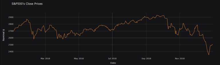
# Collect real world data for our example (for more info. see 'Part 2' bellow)
SPX = ek.get_data(instruments=".SPX", # Looking at the S&P 500, thus the ' SPX '; indecies are preceded by a full stop ' . '.
fields=["TR.CLOSEPRICE.timestamp",
"TR.CLOSEPRICE"],
parameters={'SDate': '2018-01-01',
'EDate': '2019-01-01',
'FRQ': 'D'}
)[0] # ' ek.get_data ' returns 2 objects, the 0th is the data-frame that we're interested in, thus the ' [0] '.
SPX = SPX.dropna() # We want to remove all non-business days, thus the ' .dropna() '.
We can graph our data this far:
# Import the relevent plotting libraries:
import plotly
import plotly.express
from plotly.graph_objs import *
from plotly.offline import download_plotlyjs, init_notebook_mode, plot, iplot
init_notebook_mode(connected = False)
import cufflinks
cufflinks.go_offline()
# cufflinks.set_config_file(offline = True, world_readable = True)
# seaborn is needed to plot plotly line graphs from pandas data-frames
import seaborn
import matplotlib
import matplotlib.pyplot as plt # the use of ' as ... ' (specifically here: ' as plt ') allows us to create a shorthand for a module (here: ' matplotlib.pyplot ')
%matplotlib inline
import chart_studio
chart_studio.tools.set_config_file(
plotly_domain='https://chart-studio.plotly.com',
plotly_api_domain='https://plotly.com')
for i,j in zip(["plotly", "cufflinks", "seaborn", "matplotlib"], [plotly, cufflinks, seaborn, matplotlib]):
print("The " + str(i) + " library imported in this code is version: " + j.__version__)
The plotly library imported in this code is version: 4.14.3
The cufflinks library imported in this code is version: 0.17.3
The seaborn library imported in this code is version: 0.11.1
The matplotlib library imported in this code is version: 3.2.1
pd.DataFrame(
data=list(SPX["Close Price"]),
index=SPX["Timestamp"]).iplot(
title="S&P500's Close Prices",
theme="solar", # The theme ' solar ' is what gives the graph its dark theme.
yTitle="Nominal $",
xTitle='Date')
Stationarity
We need to verify that our data is stationary (for mor informatin as to why, please see here); we can do so in Python with the Augmented Dickey-Fuller unit root test:
import statsmodels
from statsmodels.tsa.stattools import adfuller
print("The statsmodels library imported in this code is version: " + statsmodels.__version__)
def adf_table(series=SPX["Close Price"]):
"""This function returns a Pandas data-frame with the results of the
Augmented Dickey–Fuller test from the statsmodels library.
Arguments:
series (Pandas series): The series of numbers on which the test will be performed
Dependencies:
pandas 1.1.4
numpy 1.18.5
statsmodels 0.11.1
"""
_adf_stationarity_test = adfuller(x = series)
columns = [
("ADF test statistic", ""), # The ', ""' is there for the Pandas MultiIndex
("MacKinnon's approximate p-value", ""),
("The number of lags used", ""),
("Number of observations used for the ADF regression and calculation of the critical values", ""),
("Critical values for the test statistic", '1%'),
("Critical values for the test statistic", '5%'),
("Critical values for the test statistic", '10%'),
("A dummy class with results attached as attributes", "")]
columns = pd.MultiIndex.from_tuples(columns)
_adf_stationarity_test = (
list(_adf_stationarity_test[0:4]) +
[_adf_stationarity_test[4][i] for i in _adf_stationarity_test[4]] +
[_adf_stationarity_test[5]])
adf_stationarity_test = pd.DataFrame(
data=np.array(_adf_stationarity_test)[np.newaxis],
columns=columns)
return adf_stationarity_test
adf_table(series=SPX["Close Price"])
As per statsmodels, the null hypothesis of the Augmented Dickey-Fuller is that there is a unit root, with the alternative that there is no unit root. If the pvalue is above a critical size, then we cannot reject that there is a unit root. If the process has a unit root, then it is a non-stationary time series. The p-values are obtained through regression surface approximation from MacKinnon 1994, but using the updated 2010 tables. If the p-value is close to significant, then the critical values should be used to judge whether to reject the null. The autolag option and maxlag for it are described in Greene.
Since ${ADF\_t\_stat}_{SPX\_close\_prices} \approx -1.7 > \text{test statistic's critical value for the 10% significance level} \approx -2.6$, then we cannot assure the stationarity of our series and must difference it with one lag to see if we can then obtain a stationary time-series:
SPX["1d Close Price"] = SPX["Close Price"].diff() # ' 1d ' for the 1st lag's difference.
SPX
| Instrument | Timestamp | Close Price | 1d Close Price | |
| 1 | .SPX | 2018-01-02T00:00:00Z | 2695.81 | <NA> |
| 2 | .SPX | 2018-01-03T00:00:00Z | 2713.06 | 17.25 |
| 3 | .SPX | 2018-01-04T00:00:00Z | 2723.99 | 10.93 |
| 4 | .SPX | 2018-01-05T00:00:00Z | 2743.15 | 19.16 |
| 5 | .SPX | 2018-01-08T00:00:00Z | 2747.71 | 4.56 |
| ... | ... | ... | ... | ... |
| 247 | .SPX | 2018-12-24T00:00:00Z | 2351.1 | -65.52 |
| 248 | .SPX | 2018-12-26T00:00:00Z | 2467.7 | 116.6 |
| 249 | .SPX | 2018-12-27T00:00:00Z | 2488.83 | 21.13 |
| 250 | .SPX | 2018-12-28T00:00:00Z | 2485.74 | -3.09 |
| 251 | .SPX | 2018-12-31T00:00:00Z | 2506.85 | 21.11 |
adf_table(series=SPX["1d Close Price"].dropna())
|
ADF test statistic | MacKinnon's approximate p-value | The number of lags used | Number of observations used for the ADF regression and calculation of the critical values | Critical values for the test statistic | A dummy class with results attached as attributes | ||
| 1% | 5% | 10% | ||||||
| 0 | -15.63264 | 1.68E-28 | 0 | 249 | -3.456888 | -2.873219 | -2.572994 | 2240.947043 |
Since ${ADF\_t\_stat}_{SPX\_1d\_close\_prices} \approx -16 < -3 \approx \text{test statistic's critical value for the 1% significance level}$, we can regect the hypothesis that there is a unit root and presume our series to be stationary.
When working with an ARMA(2,2) with constant model, $p = 2$ and $q = 2$, we assume that $\epsilon_1 = \epsilon_2 = ... = \epsilon_{max(p,q)+p-1} = 0.$ (i.e.: $\epsilon_1 = \epsilon_2 = \epsilon_3 = 0$), and $m = max(p,q) = 2$ such that: $\hat{\bf{\beta}} = (X'X)^{-1} X' Y$ where $X = \begin{bmatrix} 1 & y_2 & y_1 \\ 1 & y_3 & y_2 \end{bmatrix} = \begin{bmatrix} 1 & SPX\_1d\_close\_prices_1 & SPX\_1d\_close\_prices_0 \\ 1 & SPX\_1d\_close\_prices_2 & SPX\_1d\_close\_prices_1 \end{bmatrix}$ and $Y = \begin{bmatrix} y_3 \\ y_4 \end{bmatrix} = \begin{bmatrix} SPX\_1d\_close\_prices_2 \\ SPX\_1d\_close\_prices_3 \end{bmatrix}$ such that:
# for ease, let's remove our 1st observation as it includes an 'NaN' value:
SPX = SPX.iloc[1:].reset_index()
SPX_Y_1 = sympy.Matrix([SPX["1d Close Price"].iloc[2],
SPX["1d Close Price"].iloc[3]]) # Remember that Python tends to be 0 indexed, so the 2nd element of our (1 indexed) list is the 1st (of its 0 indexed one)
SPX_X_1 = sympy.Matrix([[1, SPX["1d Close Price"].iloc[1],
SPX["1d Close Price"].iloc[0]],
[1, SPX["1d Close Price"].iloc[2],
SPX["1d Close Price"].iloc[1]]])
SPX_FOC_Beta_hat_1 = (((SPX_X_1.T * SPX_X_1)**(-1)) *
SPX_X_1.T * SPX_Y_1)
Thus: $\epsilon_4 = \hat{y_4} - y_4 = \hat{c} + \widehat{\phi_1} y_3 + \widehat{\phi_2} y_2 - y_4 = \begin{bmatrix} 1 & y_3 & y_2 \end{bmatrix} \hat{\beta} - y_4$ which evaluates to:
newX_1 = sympy.Matrix([1, SPX["1d Close Price"].iloc[2],
SPX["1d Close Price"].iloc[1]]).T
SPX_epsilon4 = (
newX_1 * SPX_FOC_Beta_hat_1)[0] - SPX["1d Close Price"].iloc[3] # The ' [0] ' is needed here to pick out the scalar out of the 1x1 matrix.
IMPORTANT NOTE: Invertibility When working with an ARMA(1,q) with constant model, $p = 1$ and $0 \leq q \in \mathbb{Z}$, (as per the above) $\epsilon_1 = 0$, and $m = max(p,q) = 1$, then - where $X = \begin{bmatrix} 1 & y_1 \\ \end{bmatrix} = \begin{bmatrix} 1 & SPX\_1d\_close\_prices_0 \\ \end{bmatrix}$ and $Y = \begin{bmatrix} y_2 \end{bmatrix} = \begin{bmatrix} SPX\_1d\_close\_prices_1 \end{bmatrix}$ - the estimated matrix $\hat{\beta}$ is not calculable in matrix form because the determinant of $X'X$ is 0 - as indicated by its rank). This matrix thus needs to be invertible - satisfying the condition of Invertibility (assosiated with the Moving Average part of ARMA models)Note also that this is only an issue for the 1st two steps if $q > 0$ and only the 1st step otherwise. Therefore, for ARMA(1,q) models, the 1st error term $\epsilon_{m+p}$ ought to be computed in scalar fashion.
Example 1.scalar: ARMA(1,1) with constant: Step 2:
For an ARMA(1,1) with constant model, $p = 1$ and $q = 1$. Thus, as per the above, we let $\epsilon_1 = ... = \epsilon_{m+p-1} = 0$, which is to say $\epsilon_1 = 0$, and $m = max(p,q) = 1$. The above 'Example 1.scalar: ARMA(1,1) with constant: Step 1' concluded with $\epsilon_2 = 0, \hat{c} = 0$ and $\hat{\phi_1} = \frac{y_2}{y_1}$. We now look at the FOC equation - (7) above - one step further (i.e.: where T was $m+p$ and is now $m+p+1$) :
$$ \begin{array}{ll} 0 &= \sum_{t=m+1}^{T}{ y_{t-i} \begin{Bmatrix} - y_t - \frac{1}{T} \left[ \sum_{\tau=m+1}^{T}{ - y_{\tau} + \left( \sum_{r=1}^{p} \widehat{\phi_r} y_{\tau-r} \right) }\right] + { \left( \sum_{k=1}^{p} \widehat{\phi_k} y_{t-k} \right) } \end{Bmatrix}} & \\ &= \label{eq:8} \sum_{t=m+1}^{m+p+1}{ y_{t-i} \begin{Bmatrix} - y_t - \frac{1}{m+p+1} \left[ \sum_{\tau=m+1}^{m+p+1}{ - y_{\tau} + \left( \sum_{r=1}^{p} \widehat{\phi_r} y_{\tau-r} \right) }\right] + { \left( \sum_{k=1}^{p} \widehat{\phi_k} y_{t-k} \right) } \end{Bmatrix}} & \text{ since } T = m+p+1 \tag{8} \\ &= \sum_{t=m+1}^{m+1+1}{ y_{t-1} \begin{Bmatrix} - y_t - \frac{1}{m+1+1} \left[ \sum_{\tau=m+1}^{m+1+1}{ - y_{\tau} + \left( \sum_{r=1}^{1} \widehat{\phi_r} y_{\tau-r} \right) }\right] + { \left( \sum_{k=1}^{1} \widehat{\phi_k} y_{t-k} \right) } \end{Bmatrix}} & \text{ since } p = 1 \text{ and thus } i = 1 \\ &= \sum_{t=1+1}^{1+1+1}{ y_{t-1} \begin{Bmatrix} - y_t - \frac{1}{1+1+1} \left[ \sum_{\tau=1+1}^{1+1+1}{ - y_{\tau} + \left( \sum_{r=1}^{1} \widehat{\phi_r} y_{\tau-r} \right) }\right] + { \left( \sum_{k=1}^{1} \widehat{\phi_k} y_{t-k} \right) } \end{Bmatrix}} & \text{ since } m = 1 \\ &= \sum_{t=2}^{3}{ y_{t-1} \begin{Bmatrix} - y_t - \frac{1}{3} \left[ \sum_{\tau=2}^{3}{ - y_{\tau} + \left( \sum_{r=1}^{1} \widehat{\phi_r} y_{\tau-r} \right) }\right] + { \left( \sum_{k=1}^{1} \widehat{\phi_k} y_{t-k} \right) } \end{Bmatrix}} & \\ &= y_1 \begin{Bmatrix} - y_2 - \frac{1}{3} \left[ - y_2 + \left( \widehat{\phi_1} y_1 \right) - y_3 + \left( \widehat{\phi_1} y_2 \right) \right] + \left( \widehat{\phi_1} y_1 \right) \end{Bmatrix} \\ & \text{ } + y_2 \begin{Bmatrix} - y_3 - \frac{1}{3} \left[ - y_2 + \left( \widehat{\phi_1} y_1 \right) - y_3 + \left( \widehat{\phi_1} y_2 \right) \right] + \left( \widehat{\phi_1} y_{2} \right) \end{Bmatrix} \end{array} $$
y1, y2, y3, phi1 = sympy.symbols("y_1, y_2, y_3, \phi_1")
equation = y1*(-y2 - ((1/3)*(-y2 + phi1*y1 - y3 + phi1*y2)) + phi1*y1
) + y2*(-y3 - ((1/3)*(-y2 + phi1*y1 - y3 + phi1*y2)) + phi1*y2)
phi_1_equation = sympy.solve(equation, phi1)[0]
phi_1_equation
$\displaystyle \frac{y_{1} y_{2} - 0.5 y_{1} y_{3} - 0.5 y_{2}^{2} + y_{2} y_{3}}{y_{1}^{2} - y_{1} y_{2} + y_{2}^{2}}$
Thus $\hat{\phi_1} = \frac{y_1 y_2 - 0.5 y_1 y_3 - 0.5 {y_2}^2 + y_2 y_3}{{y_1}^2 - y_1 y_2 + {y_2}^2}$ and, as per (6) which becomes $$ \begin{array}{ll} \widehat{c} &= - \frac{1}{T} \sum_{t=m+1}^{T}{ \left[ - y_t + \left( \sum_{r=1}^{p} \widehat{\phi_r} y_{t-r} \right) + \left( \sum_{j=1}^{q} \widehat{\psi_j} \epsilon_{t-j} \right) \right] } & \\ &= - \frac{1}{3} \sum_{t=2}^{3}{ \left[ - y_t + \left( \sum_{r=1}^{1} \widehat{\phi_r} y_{t-r} \right) + \left( \sum_{j=1}^{1} \widehat{\psi_j} \epsilon_{t-j} \right) \right] } & \text{ since } p=q=m=1 \text{ and thus } T = m+p+1 = 3 \\ &= - \frac{1}{3} \sum_{t=2}^{3}{ \left[ - y_t + \left(\widehat{\phi_1} y_{t-1} \right) \right] } & \text{ since } \epsilon_1 = \epsilon_2 = 0 \\ &= - \frac{1}{3} \begin{Bmatrix} \left[ - y_2 + \left(\widehat{\phi_1} y_1 \right) \right] + \left[ - y_3 + \left(\widehat{\phi_1} y_2 \right) \right] \end{Bmatrix} & \\ &= - \frac{1}{3} \left[ \widehat{\phi_1} \left( y_1 + y_2 \right) - y_2 - y_3 \right] & \end{array} $$
c_hat_equation = (-1/3)*(phi_1_equation*(y1+y2)-y2-y3)
c_hat_equation
$\displaystyle 0.333333333333333 y_{2} + 0.333333333333333 y_{3} - \frac{0.333333333333333 \left(y_{1} + y_{2}\right) \left(y_{1} y_{2} - 0.5 y_{1} y_{3} - 0.5 y_{2}^{2} + y_{2} y_{3}\right)}{y_{1}^{2} - y_{1} y_{2} + y_{2}^{2}}$
Thus $\hat{c} = \frac{y_2 + y_3}{3} - \frac{y_1 + y_2}{3} \frac{y_1 y_2 - 0.5 y_1 y_3 - 0.5 {y_2}^2 + y_2 y_3}{y_1^2 - y_1 y_2 + y_2^2}$
Now: $\epsilon_3 = \hat{y_3} - y_3 = \hat{c} + \hat{\phi_1} y_2 + \hat{\psi_1} \epsilon_2 - y_3$
y_hat_3 = c_hat_equation + phi_1_equation * y2
epsilon_3 = y_hat_3 - y3
epsilon_3
$\displaystyle 0.333333333333333 y_{2} + \frac{y_{2} \left(y_{1} y_{2} - 0.5 y_{1} y_{3} - 0.5 y_{2}^{2} + y_{2} y_{3}\right)}{y_{1}^{2} - y_{1} y_{2} + y_{2}^{2}} - 0.666666666666667 y_{3} - \frac{0.333333333333333 \left(y_{1} + y_{2}\right) \left(y_{1} y_{2} - 0.5 y_{1} y_{3} - 0.5 y_{2}^{2} + y_{2} y_{3}\right)}{y_{1}^{2} - y_{1} y_{2} + y_{2}^{2}}$
y_hat_3_evaluated = y_hat_3.subs(y1, SPX["1d Close Price"].iloc[0]
).subs(y2, SPX["1d Close Price"].iloc[1]
).subs(y3, SPX["1d Close Price"].iloc[2])
epsilon_3_evaluated = y_hat_3_evaluated - SPX["1d Close Price"].iloc[2] # Remember, y3 is the 2nd SPX_close_prices element since the latter is 0 indexed.
epsilon_3_evaluated
−7.96667082813824
From 'Example 1.scalar: ARMA(1,1) with constant: Step 1', we know that $\epsilon_2 = 0$
Now that we have our value for $\epsilon_{m+p}$, the MA part of our model cannot be ignored. Since since $\epsilon_1, \epsilon_2, ..., \epsilon_{m+p-1} = 0$, and $\epsilon_{m+p} \in \mathbb{R}$,
$$ \begin{bmatrix} y_{m + 1} \\ y_{m + 2} \\ ... \\ y_{m + p} \end{bmatrix} = \begin{bmatrix} 1 & y_{m} & y_{m-1} & ... & y_{m-p+1} & \epsilon_{m} & \epsilon_{m-1} & ... & \epsilon_{m-q+1} \\ 1 & y_{m+1} & y_{m} & ... & y_{m-p+2} & \epsilon_{m+1} & \epsilon_{m} & ... & \epsilon_{m-q+2} \\ ... & ... & ... & ... & ... & ... & ... & ... & ... \\ 1 & y_{m+p-1} & y_{m+p-2} & ... & y_{m} & \epsilon_{m+p-1} & \epsilon_{m+p-2} & ... & \epsilon_{m} \end{bmatrix} \begin{bmatrix} c \\ \phi_1 \\ ... \\ \phi_p \\ \psi_1 \\ ... \\ \psi_q \end{bmatrix} + \begin{bmatrix} \epsilon_{m + 1} \\ \epsilon_{m + 2} \\ ... \\ \epsilon_{m + p} \end{bmatrix} $$becomes
$$ \begin{bmatrix} y_{m + 1} \\ y_{m + 2} \\ ... \\ y_{m + p} \\ y_{m + p + 1} \end{bmatrix} = \begin{bmatrix} 1 & y_{m} & y_{m-1} & ... & y_{m-p+1} & 0 \\ 1 & y_{m+1} & y_{m} & ... & y_{m-p+2} & 0 \\ ... & ... & ... & ... & ... & ... & \\ 1 & y_{m+p-1} & y_{m+p-2} & ... & y_{m} & 0 \\ 1 & y_{m+p} & y_{m+p-1} & ... & y_{m+1} & \epsilon_{m+p} \end{bmatrix} \begin{bmatrix} c \\ \phi_1 \\ ... \\ \phi_p \\ \psi_1 \end{bmatrix} + \begin{bmatrix} 0 \\ ... \\ 0 \\\epsilon_{m + p} \\ \epsilon_{m + p + 1} \end{bmatrix} $$FOC equations equate to $\hat{\bf{\beta}} = (X'X)^{-1} X' \hat{Y}$ which - using actual $y$ values (i.e.: $Y$ as opposed to $\hat{Y}$) - renders: $\hat{\bf{\beta}} = (X'X)^{-1} X' Y$.
We revert back to scalars: now that we have our estimate values, we can compute $\hat{y}_{max(p,q)+p+1} = \hat{c} + \left( \sum_{i=1}^{p}\hat{\phi_i} y_{max(p,q)+p-i+1} \right) + \hat{\psi_1} \epsilon_{max(p,q)+p}$, from which we can compute $\epsilon_{max(p,q)+p+1} = \hat{y}_{max(p,q)+p+1} - y_{max(p,q)+p+1}$, i.e: $$\epsilon_{m+p+1} = \hat{y}_{m+p+1} - y_{m+p+1}$$
SPX_Y_2 = sympy.Matrix([SPX["1d Close Price"].iloc[i] for i in [2, 3, 4]]) # Remember that Python tends to be 0 indexed, so the 2nd element of our (1 indexed) list is the 1st (of its 0 indexed one)
SPX_X_2 = sympy.Matrix(
[[1] + [SPX["1d Close Price"].iloc[i] for i in [1, 0]] + [0], # ' [1] + ' inserts the integer ' 1 ' at the start of the list; similarly to ' [0] ' a the end.
[1] + [SPX["1d Close Price"].iloc[i] for i in [2, 1]] + [0],
[1] + [SPX["1d Close Price"].iloc[i] for i in [3, 2]] + [SPX_epsilon4]])
SPX_FOC_Beta_hat_2 = ((SPX_X_2.T * SPX_X_2)**(-1)) * SPX_X_2.T * SPX_Y_2
newX_2 = sympy.Matrix([1] + [SPX["1d Close Price"].iloc[i] for i in [3, 2]] + [SPX_epsilon4]).T
SPX_epsilon5 = (newX_2 * SPX_FOC_Beta_hat_2)[0] - SPX["1d Close Price"].iloc[4] # The ' [0] ' is needed here to pick out the scalar out of the 1x1 matrix.
SPX_epsilon5
−32.3306317768573
Step 3: Compute $\epsilon_{max(p,q)+p+2}$ onwards
In Scalar Terms
You may chose to continue itteratively in scalar terms, continuing the trend set hitherto.
In Matrix Terms
All we have to do is continue our previous setu whereby $\epsilon_{m+p+2} = \hat{y}_{m+p+2} - y_{m+p+2}$ and $\epsilon_{m+p+3} = \hat{y}_{m+p+3} - y_{m+p+3}$ and on...
SPX
| index | Instrument | Timestamp | Close Price | 1d Close Price | |
| 0 | 2 | .SPX | 2018-01-03T00:00:00Z | 2713.06 | 17.25 |
| 1 | 3 | .SPX | 2018-01-04T00:00:00Z | 2723.99 | 10.93 |
| 2 | 4 | .SPX | 2018-01-05T00:00:00Z | 2743.15 | 19.16 |
| 3 | 5 | .SPX | 2018-01-08T00:00:00Z | 2747.71 | 4.56 |
| 4 | 6 | .SPX | 2018-01-09T00:00:00Z | 2751.29 | 3.58 |
| ... | ... | ... | ... | ... | ... |
| 245 | 247 | .SPX | 2018-12-24T00:00:00Z | 2351.1 | -65.52 |
| 246 | 248 | .SPX | 2018-12-26T00:00:00Z | 2467.7 | 116.6 |
| 247 | 249 | .SPX | 2018-12-27T00:00:00Z | 2488.83 | 21.13 |
| 248 | 250 | .SPX | 2018-12-28T00:00:00Z | 2485.74 | -3.09 |
| 249 | 251 | .SPX | 2018-12-31T00:00:00Z | 2506.85 | 21.11 |
250 rows × 5 columns
SPX_Y_3 = sympy.Matrix([SPX["1d Close Price"].iloc[i] for i in [2, 3, 4, 5]]) # Remember that Python tends to be 0 indexed, so the 2nd element of our (1 indexed) list is the 1st (of its 0 indexed one)
SPX_X_3 = sympy.Matrix(
[[1] + [SPX["1d Close Price"].iloc[i] for i in [1, 0]] + [0] + [0], # ' [1] + ' inserts the integer ' 1 ' at the start of the list; similarly to ' [0] ' a the end.
[1] + [SPX["1d Close Price"].iloc[i] for i in [2, 1]] + [0] + [0],
[1] + [SPX["1d Close Price"].iloc[i] for i in [3, 2]] + [SPX_epsilon4] + [0],
[1] + [SPX["1d Close Price"].iloc[i] for i in [4, 3]] + [SPX_epsilon4] + [SPX_epsilon5]])
SPX_FOC_Beta_hat_3 = ((SPX_X_3.T * SPX_X_3)**(-1)) * SPX_X_3.T * SPX_Y_3
newX_3 = sympy.Matrix([1] + [SPX["1d Close Price"].iloc[i] for i in [4, 3]] + [SPX_epsilon4] + [SPX_epsilon5]).T
SPX_epsilon6 = (newX_3 * SPX_FOC_Beta_hat_3)[0] - SPX["1d Close Price"].iloc[5] # The ' [0] ' is needed here to pick out the scalar out of the 1x1 matrix.
SPX_epsilon6
−38.685458159182
c, p, q = True, 3, 2
m = max(p, q)
Setting up empty lists:
SPX_X, SPX_Y, SPX_epsilon, SPX_FOC_Beta_hat, _SPX_epsilon, Timestamp, SPX_Y_hat = [], [], [], [], [], [], []
Let's set '$C$' to be 0 if there is no constant:
if c is True:
C = 1
elif c is False:
C = 0
else:
print("argument 'c' as to be Boolean; either 'True' or 'False'.")
Generalising: Step 1: $SPX\_Y$
We will permute through a list starting at 0, call it ' a '. We can now define $ SPX\_Y\_component_a = \begin{bmatrix} y_{m + 1} \\ y_{m + 2} \\ ... \\ y_{m + p + a} \end{bmatrix}= \begin{bmatrix} SPX\_1d\_close\_prices_m \\ SPX\_1d\_close\_prices_{m + 1} \\ ... \\ SPX\_1d\_close\_prices_{m + p + a - 1} \end{bmatrix} $ for $0 \leq a \in \mathbb{Z}$ such that we may have a (psudo) matrix $ SPX\_Y = \begin{bmatrix} SPX\_Y\_component_0 \\ SPX\_Y\_component_1 \\ ... \\ SPX\_Y\_component_{T-1} \end{bmatrix} $. 'Psudo' because it is actually a Python list of lists, not a Matrix. As a matter of fact, througout this investigation, I will be using Python lists instead of Sympy matricies, only because they are simpler to manipulate; I will convert them when nessesary. The 'T-1' above is there because we have SPX_close_prices data from point 1 to T and $SPX\_Y$ is 0 indexed.
for a in range(10):
SPX_Y_component = [SPX["1d Close Price"].iloc[b]
for b in [m+d for d in range(a+p)]] # This will start at the 'm'th.
Timestamp_component = [SPX["Timestamp"].iloc[b]
for b in [m+d for d in range(a+p)]]
SPX_Y.append(SPX_Y_component)
Timestamp.append(Timestamp_component)
Let $\epsilon_{m+t} = \hat{y}_{m+t} - y_{m+t} = \hat{y}_{m+t} - SPX\_1d\_close\_prices_{m+t-1}$ $ \forall $ $ 0 > t \leq T $ and $ t \in \mathbb{Z}$ up to the appropriate end of our $SPX\_1d\_close\_prices$ data-set and: $$ \begin{array}{ll} SPX\_X\_component_0 &= \begin{Bmatrix} \begin{bmatrix} y_m & y_{m - 1} & ... & y_{m - p + 1} \end{bmatrix} & \text{ for a model with no constant } \\ \begin{bmatrix} 1 & y_m & y_{m - 1} & ... & y_{m - p + 1} \end{bmatrix} & \text{ for a model with a constant } \end{Bmatrix} \\ &= \begin{Bmatrix} \begin{bmatrix} SPX\_1d\_close\_prices_{m-1} & SPX\_1d\_close\_prices_m & ... & SPX\_1d\_close\_prices_{m - p} \end{bmatrix} & \text{ for a model with no constant } \\ \begin{bmatrix} 1 & SPX\_1d\_close\_prices_{m-1} & SPX\_1d\_close\_prices_m & ... & SPX\_1d\_close\_prices_{m - p} \end{bmatrix} & \text{ for a model with a constant } \end{Bmatrix} \end{array} $$
and $$ \begin{array}{ll} SPX\_X\_component_1 &= \begin{Bmatrix} \begin{bmatrix} y_m & y_{m - 1} & ... & y_{m - p + 1} & 0 \\ y_{m+1} & y_{m} & ... & y_{m - p + 2} & \epsilon_{m+1} \end{bmatrix} & \text{ for a model with no constant } \\ \begin{bmatrix} 1 & y_m & y_{m-1} & ... & y_{m - p + 1} & 0 \\ 1 & y_{m+1} & y_{m} & ... & y_{m - p + 2} & \epsilon_{m+1} \end{bmatrix} & \text{ for a model with a constant } \end{Bmatrix} \\ &= \begin{Bmatrix} \begin{bmatrix} SPX\_1d\_close\_prices_{m-1} & SPX\_1d\_close\_prices_{m-2} & ... & SPX\_1d\_close\_prices_{m - p} & 0 \\ SPX\_1d\_close\_prices_{m} & SPX\_1d\_close\_prices_{m-1} & ... & SPX\_1d\_close\_prices_{m - p + 1} & \epsilon_{m+1} \end{bmatrix} & \text{ for a model with no constant } \\ \begin{bmatrix} 1 & SPX\_1d\_close\_prices_{m-1} & SPX\_1d\_close\_prices_{m-2} & ... & SPX\_1d\_close\_prices_{m - p} & 0 \\ 1 & SPX\_1d\_close\_prices_{m} & SPX\_1d\_close\_prices_{m-1} & ... & SPX\_1d\_close\_prices_{m - p + 1} & \epsilon_{m+1} \end{bmatrix} & \text{ for a model with a constant } \end{Bmatrix} \end{array} $$
and we let $$ \begin{array}{ll} SPX\_X\_component_2 &= \begin{Bmatrix} \begin{bmatrix} y_m & y_{m - 1} & ... & y_{m - p + 1} & 0 & 0 \\ y_{m+1} & y_{m} & ... & y_{m - p + 2} & \epsilon_{m+1} & 0 \\ y_{m+2} & y_{m+1} & ... & y_{m - p + 3} & \epsilon_{m+2} & \epsilon_{m+1} \end{bmatrix} & \text{ for a model with no constant } \\ \begin{bmatrix} 1 & y_m & y_{m-1} & ... & y_{m - p + 1} & 0 & 0 \\ 1 & y_{m+1} & y_{m} & ... & y_{m - p + 2} & \epsilon_{m+1} & 0 \\ 1 & y_{m+2} & y_{m+1} & ... & y_{m - p + 3} & \epsilon_{m+2} & \epsilon_{m+1} & 0 \end{bmatrix} & \text{ for a model with a constant } \end{Bmatrix} \\ &= \begin{Bmatrix} \begin{bmatrix} SPX\_1d\_close\_prices_{m-1} & SPX\_1d\_close\_prices_{m-2} & ... & SPX\_1d\_close\_prices_{m - p} & 0 & 0 \\ SPX\_1d\_close\_prices_{m} & SPX\_1d\_close\_prices_{m-1} & ... & SPX\_1d\_close\_prices_{m - p + 1} & \epsilon_{m+1} & 0 \\ SPX\_1d\_close\_prices_{m+1} & SPX\_1d\_close\_prices_{m} & ... & SPX\_1d\_close\_prices_{m - p + 2} & \epsilon_{m+2} & \epsilon_{m+1} \end{bmatrix} & \text{ for a model with no constant } \\ \begin{bmatrix} 1 & SPX\_1d\_close\_prices_{m-1} & SPX\_1d\_close\_prices_{m-2} & ... & SPX\_1d\_close\_prices_{m - p} & 0 & 0 \\ 1 & SPX\_1d\_close\_prices_{m} & SPX\_1d\_close\_prices_{m-1} & ... & SPX\_1d\_close\_prices_{m - p + 1} & \epsilon_{m+1} & 0 \\ 1 & SPX\_1d\_close\_prices_{m+1} & SPX\_1d\_close\_prices_{m} & ... & SPX\_1d\_close\_prices_{m - p + 2} & \epsilon_{m+2} & \epsilon_{m+1} \end{bmatrix} & \text{ for a model with a constant } \end{Bmatrix} \end{array} $$
From now on, we will only look at the case of a model with a constant. This is to save space and reduce dificulties anyone may have in reading through the maths this far all while investigating the most complex of the two cases.
We continue like this untill $q$ - MA components - such that $$ \begin{array}{ll} SPX\_X\_component_q &= \begin{bmatrix} 1 & y_m & y_{m - 1} & ... & y_{m - p + 1} & 0 & 0 & 0 & ... & 0 \\ 1 & y_{m+1} & y_{m} & ... & y_{m - p + 2} & \epsilon_{m+1} & 0 & 0 & ... & 0 \\ 1 & y_{m+2} & y_{m+1} & ... & y_{m - p + 3} & \epsilon_{m+2} & \epsilon_{m+1} & 0 & ... & 0 \\ ... & ... & ... & ... & ... & ... & ... & ... & ... & ... \\ 1 & y_{m+q} & y_{m+q-1} & ... & y_{m+q-p+1} & \epsilon_{m+q} & \epsilon_{m+q-1} & \epsilon_{m+q-2} & ... & \epsilon_{m+1} \end{bmatrix} \\ &= \begin{bmatrix} 1 & SPX\_1d\_close\_prices_{m-1} & SPX\_1d\_close\_prices_{m-2} & ... & SPX\_1d\_close\_prices_{m-p} & 0 & 0 & 0 & ... & 0 \\ 1 & SPX\_1d\_close\_prices_{m} & SPX\_1d\_close\_prices_{m-1} & ... & SPX\_1d\_close\_prices_{m-p+1} & \epsilon_{m+1} & 0 & 0 & ... & 0 \\ 1 & SPX\_1d\_close\_prices_{m+1} & SPX\_1d\_close\_prices_{m} & ... & SPX\_1d\_close\_prices_{m-p+2} & \epsilon_{m+2} & \epsilon_{m+1} & 0 & ... & 0 \\ ... & ... & ... & ... & ... & ... & ... & ... & ... & ... \\ 1 & SPX\_1d\_close\_prices_{m+q-1} & SPX\_1d\_close\_prices_{m+q-2} & ... & SPX\_1d\_close\_prices_{m+q-p} & \epsilon_{m+q} & \epsilon_{m+q-1} & \epsilon_{m+q-2} & ... & \epsilon_{m+1} \end{bmatrix} \end{array} $$
before moving onwards: $$ \begin{array}{ll} SPX\_X\_component_{q+1} &= \begin{bmatrix} 1 & y_m & y_{m - 1} & ... & y_{m - p + 1} & 0 & 0 & 0 & ... & 0 \\ 1 & y_{m+1} & y_{m} & ... & y_{m - p + 2} & \epsilon_{m+1} & 0 & 0 & ... & 0 \\ 1 & y_{m+2} & y_{m+1} & ... & y_{m - p + 3} & \epsilon_{m+2} & \epsilon_{m+1} & 0 & ... & 0 \\ ... & ... & ... & ... & ... & ... & ... & ... & ... & ... \\ 1 & y_{m+q} & y_{m+q-1} & ... & y_{m+q-p+1} & \epsilon_{m+q} & \epsilon_{m+q-1} & \epsilon_{m+q-2} & ... & \epsilon_{m+1} \\ 1 & y_{m+q+1} & y_{m+q} & ... & y_{m+q-p+2} & \epsilon_{m+q+1} & \epsilon_{m+q} & \epsilon_{m+q-1} & ... & \epsilon_{m+2} \end{bmatrix} \\ &= \begin{bmatrix} 1 & SPX\_1d\_close\_prices_{m-1} & SPX\_1d\_close\_prices_{m-2} & ... & SPX\_1d\_close\_prices_{m-p} & 0 & 0 & 0 & ... & 0 \\ 1 & SPX\_1d\_close\_prices_{m} & SPX\_1d\_close\_prices_{m-1} & ... & SPX\_1d\_close\_prices_{m-p+1} & \epsilon_{m+1} & 0 & 0 & ... & 0 \\ 1 & SPX\_1d\_close\_prices_{m+1} & SPX\_1d\_close\_prices_{m} & ... & SPX\_1d\_close\_prices_{m-p+2} & \epsilon_{m+2} & \epsilon_{m+1} & 0 & ... & 0 \\ ... & ... & ... & ... & ... & ... & ... & ... & ... & ... \\ 1 & SPX\_1d\_close\_prices_{m+q-1} & SPX\_1d\_close\_prices_{m+q-2} & ... & SPX\_1d\_close\_prices_{m+q-p} & \epsilon_{m+q} & \epsilon_{m+q-1} & \epsilon_{m+q-2} & ... & \epsilon_{m+1} \\ 1 & SPX\_1d\_close\_prices_{m+q} & SPX\_1d\_close\_prices_{m+q-1} & ... & SPX\_1d\_close\_prices_{m+q-p+1} & \epsilon_{m+q+1} & \epsilon_{m+q} & \epsilon_{m+q-1} & ... & \epsilon_{m+2} \end{bmatrix} \end{array} $$
up to $T-1$. (Why not up to $T$? Because we need to compare the regressor $SPX\_X\_component_{T-1}$ with the regressand $SPX\_Y\_component_{T-1}$ since they are both 0 indexed:) $$ \begin{array}{ll} SPX\_X\_component_{T-1} &= \begin{bmatrix} 1 & y_m & y_{m - 1} & ... & y_{m - p + 1} & 0 & 0 & 0 & ... & 0 \\ 1 & y_{m+1} & y_{m} & ... & y_{m - p + 2} & \epsilon_{m+1} & 0 & 0 & ... & 0 \\ 1 & y_{m+2} & y_{m+1} & ... & y_{m - p + 3} & \epsilon_{m+2} & \epsilon_{m+1} & 0 & ... & 0 \\ ... & ... & ... & ... & ... & ... & ... & ... & ... & ... \\ 1 & y_{m+q} & y_{m+q-1} & ... & y_{m+q-p+1} & \epsilon_{m+q} & \epsilon_{m+q-1} & \epsilon_{m+q-2} & ... & \epsilon_{m+1} \\ ... & ... & ... & ... & ... & ... & ... & ... & ... & ... \\ 1 & y_{T-1} & y_{T-2} & ... & y_{T-p} & \epsilon_{T-1} & \epsilon_{T-2} & \epsilon_{T-3} & ... & \epsilon_{T-q} \end{bmatrix} \\ &= \begin{bmatrix} 1 & SPX\_1d\_close\_prices_{m-1} & SPX\_1d\_close\_prices_{m-2} & ... & SPX\_1d\_close\_prices_{m-p} & 0 & 0 & 0 & ... & 0 \\ 1 & SPX\_1d\_close\_prices_{m} & SPX\_1d\_close\_prices_{m-1} & ... & SPX\_1d\_close\_prices_{m-p+1} & \epsilon_{m+1} & 0 & 0 & ... & 0 \\ 1 & SPX\_1d\_close\_prices_{m+1} & SPX\_1d\_close\_prices_{m} & ... & SPX\_1d\_close\_prices_{m-p+2} & \epsilon_{m+2} & \epsilon_{m+1} & 0 & ... & 0 \\ ... & ... & ... & ... & ... & ... & ... & ... & ... & ... \\ 1 & SPX\_1d\_close\_prices_{m+q-1} & SPX\_1d\_close\_prices_{m+q-2} & ... & SPX\_1d\_close\_prices_{m+q-p} & \epsilon_{m+q} & \epsilon_{m+q-1} & \epsilon_{m+q-2} & ... & \epsilon_{m+1} \\ ... & ... & ... & ... & ... & ... & ... & ... & ... & ... \\ 1 & SPX\_1d\_close\_prices_{T-2} & SPX\_1d\_close\_prices_{T-3} & ... & SPX\_1d\_close\_prices_{T-p-1} & \epsilon_{T-1} & \epsilon_{T-2} & \epsilon_{T-3} & ... & \epsilon_{T-q} \end{bmatrix} \end{array} $$
Finally - we can put them all together in the Python list of lists / psudo matrix: $ SPX\_X = \begin{bmatrix} SPX\_X\_component_0 \\ SPX\_X\_component_1 \\ ... \\ SPX\_X\_component_{T-1} \end{bmatrix} $
There are 4 senarios we need to code for where $q>0<p$:
- $1^{st}$: ARMA(p,0)
- $2^{nd}$: ARMA(p,1)
- $3^{rd}$: ARMA(1,q)
- $4^{th}$: ARMA(0,q): Unfortunutally, pure MA models are too different to arange for in the way described in this article. Their parameters often need to be estimated via computational methods as opposed to empirical ones. There is an empirical solution out there (Denise R. Osborn's Annals of Economic and Social Measurement, Volume 5, number 1: Maximum Likelihood Estimation of Moving Average Processes), but it would require an article of its own. Suffice to say that if you wish to build an MA model, the existing python libraries tend to be enough.
SPX_Y_component = [SPX["1d Close Price"].iloc[b] for b in [2+d for d in range(2+2)]]
SPX_Y_component
[19.16000000000031, 4.559999999999945, 3.5799999999999272, -3.0599999999999454]
SPX_Y_hat_component_Timestamp = SPX["Timestamp"].iloc[2+2+2-1]
SPX_Y_hat_component_Timestamp
'2018-01-10T00:00:00Z'
SPX.head(10)
| index | Instrument | Timestamp | Close Price | 1d Close Price | |
| 0 | 2 | .SPX | 2018-01-03T00:00:00Z | 2713.06 | 17.25 |
| 1 | 3 | .SPX | 2018-01-04T00:00:00Z | 2723.99 | 10.93 |
| 2 | 4 | .SPX | 2018-01-05T00:00:00Z | 2743.15 | 19.16 |
| 3 | 5 | .SPX | 2018-01-08T00:00:00Z | 2747.71 | 4.56 |
| 4 | 6 | .SPX | 2018-01-09T00:00:00Z | 2751.29 | 3.58 |
| 5 | 7 | .SPX | 2018-01-10T00:00:00Z | 2748.23 | -3.06 |
| 6 | 8 | .SPX | 2018-01-11T00:00:00Z | 2767.56 | 19.33 |
| 7 | 9 | .SPX | 2018-01-12T00:00:00Z | 2786.24 | 18.68 |
| 8 | 10 | .SPX | 2018-01-16T00:00:00Z | 2776.42 | -9.82 |
| 9 | 11 | .SPX | 2018-01-17T00:00:00Z | 2802.56 | 26.14 |
p, q, a = 2, 6, 10
m = max(p, q)
[[f+g for g in range(p)][::-1] for f in range(m-p, m+a)]
[[5, 4],
[6, 5],
[7, 6],
[8, 7],
[9, 8],
[10, 9],
[11, 10],
[12, 11],
[13, 12],
[14, 13],
[15, 14],
[16, 15]]
p = 2
q = 1
c = True
m = max(p, q)
SPX_X, SPX_Y, SPX_epsilon, SPX_FOC_Beta_hat, _SPX_epsilon, SPX_Y_hat, SPX_Y_hat_Timestamp = [], [], [], [], [], [], []
if c is True: C = 1
elif c is False: C = 0
else: print("argument 'c' as to be Boolean; either 'True' or 'False'.")
for a in range(200):
# 1st: Set up the Y matrix:
SPX_Y_component = [SPX["1d Close Price"].iloc[b]
for b in [m+d for d in range(a+p)]] # This will start at the 'm'th. Remember also that this range goes up to - but does not include the 'm+a+p'th element of the 0 indexed ' SPX["1d Close Price"] ' pandas data-frame.
SPX_Y_hat_component_Timestamp = SPX["Timestamp"].iloc[m+a+p-1] # ' -1 ' because it is 0 indexed
# # You can check the timestamp in the senario where q is 1 and p & a is 2:
# SPX_Y_component_test = [SPX["1d Close Price"].iloc[b] for b in [2+d for d in range(2+2)]]
# display(SPX_Y_component_test)
# SPX_Y_hat_component_Timestamp_test = SPX["Timestamp"].iloc[2+2+2-1]
# display(SPX_Y_hat_component_Timestamp_test)
# 2nd: Setup the AR component of our X matrix used in the FOC equation:
SPX_X_component = []
for f in range(m-p, m+a): # ' m-p ' is there in case q > p.
F = [f+g for g in range(p)][::-1] # ' [::-1] ' allows us to go backwards through our list. Note that using ' range(p) ' starts at 0 and ends at p-1 inclusive.
# # You can check F via the below:
# p, q, a = 2, 6, 10
# m = max(p, q)
# [[f+g for g in range(p)][::-1] for f in range(m-p, m+a)]
SPX_X_component.append(
[SPX["1d Close Price"].iloc[h] for h in F] + min(q, a)*[0]) # ' min(q,a)*[0] ' adds 0s at the end of our rows, only enough for our MA components.
if c is True:
SPX_X_component[f-m+p] = [1] + SPX_X_component[f-m+p] # The ' -m+p ' is just there to normalise the index of our list; note that ' f-m+p ' has to start at 0.
if a == 0:
_SPX_epsilon = [[0]*j for j in range(1, p+1)]
elif a > 0:
_SPX_epsilon.append([0]*p + SPX_epsilon[::-1][0:min(q, a+1)])
for col in range(p+C, len(SPX_X_component[0])):
for row in range(p, len(SPX_X_component)):
try:
if SPX_X_component[row][col] == 0:
SPX_X_component[row][col] = _SPX_epsilon[row][col-C]
except:
pass
SPX_newX_component = SPX_X_component[-1]
SPX_X_component_M = sympy.Matrix(SPX_X_component)
# If p = 1, we have to use our scalar method for the following 2 steps:
if p == 1 and a == 0:
if c is True:
SPX_FOC_Beta_hat_component = [0,
SPX["1d Close Price"].iloc[m+p+a-1] /
SPX["1d Close Price"].iloc[m+p+a-2]]
SPX_epsilon_component = 0
SPX_Y_hat_component = SPX["1d Close Price"].iloc[m+p+a-1]
else:
if p == 1 and a == 1:
SPX_FOC_Beta_hat_component = [
phi_1_equation.subs(y1, SPX["1d Close Price"].iloc[m-p]
).subs(y2, SPX["1d Close Price"].iloc[m-p+1]
).subs(y3, SPX["1d Close Price"].iloc[m-p+2])]
if c is True:
SPX_FOC_Beta_hat_component = [
c_hat_equation.subs(y1, SPX["1d Close Price"].iloc[m-p]).subs(
y2, SPX["1d Close Price"].iloc[m-p+1]).subs(
y3, SPX["1d Close Price"].iloc[m-p+2])] + SPX_FOC_Beta_hat_component
SPX_FOC_Beta_hat_component = sympy.Matrix(SPX_FOC_Beta_hat_component)
if q > 0:
SPX_newX_component = SPX_newX_component[:-1] # We need to ignore the previous MA part since epsilon was 0 then
elif p == 1 and q > 0 and a <= q: # We need to ignore the previous MA part since epsilon was 0 then:
_SPX_X_component_M = SPX_X_component_M
_SPX_X_component_M.col_del(-1) # We are deleting this column as we are looking at an extra case where epsilon = 0.
SPX_FOC_Beta_hat_component = (
((_SPX_X_component_M.T * _SPX_X_component_M)**(-1)) *
_SPX_X_component_M.T * sympy.Matrix(SPX_Y_component))
SPX_newX_component = SPX_newX_component[:-1]
else:
SPX_FOC_Beta_hat_component = (((
SPX_X_component_M.T *SPX_X_component_M)**(-1)) *
SPX_X_component_M.T * sympy.Matrix(SPX_Y_component))
SPX_Y_hat_component = (sympy.Matrix(SPX_newX_component).T * SPX_FOC_Beta_hat_component)[0]
SPX_epsilon_component = SPX["1d Close Price"].iloc[m+p+a-1] - SPX_Y_hat_component
# Note that ' SPX["1d Close Price"].iloc[m+p+a-1] ' is the same as ' SPX["1d Close Price"][SPX["Timestamp"] == SPX_Y_hat_component_Timestamp] '.
SPX_X.append(SPX_X_component)
SPX_Y.append(SPX_Y_component)
SPX_FOC_Beta_hat.append(SPX_FOC_Beta_hat_component)
SPX_epsilon.append(SPX_epsilon_component)
SPX_Y_hat_Timestamp.append(SPX_Y_hat_component_Timestamp)
SPX_Y_hat.append(SPX_Y_hat_component)
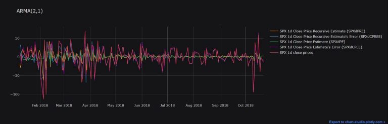
# Our method above recursively computed elements, but now that we've trained our model up to max(a), we can use our elements to compute our non-recursive estimates:
non_recursive_SPX_Y_hat = (SPX_X_component_M * SPX_FOC_Beta_hat_component)[-len(SPX_Y_hat):] # both elements on the right-hand-side are the latest in our loop through ' a ' above. The ' -len(SPX_Y_hat) ' gets us the last x elements, where x = len(SPX_Y_hat)
SPX_Y_hat_df = pd.DataFrame(index = SPX_Y_hat_Timestamp,
data = {
"SPX 1d Close Price Recursive Estimate (SPXdPRE)": [float(i) for i in SPX_Y_hat], # This 'float' business is needed here to convert our data in a way that pyplot "enjoys".
"SPX 1d Close Price Recursive Estimate's Error (SPXdCPREE)": [float(i) for i in SPX_epsilon],
"SPXdPRE - SPXdCPREE": [float(SPX_Y_hat[k] + SPX_epsilon[k]) for k in range(len(SPX_Y_hat))],
"SPX 1d Close Price Estimate (SPXdPE)": [float(i) for i in non_recursive_SPX_Y_hat],
"SPX 1d Close Price Estimate's Error (SPXdCPEE)": [float(i) - float(j) for i, j in zip(SPX["1d Close Price"].iloc[m+p-1 : m+p-1+len(SPX_Y_hat)], non_recursive_SPX_Y_hat)],
"SPX 1d close prices Timestamp": list(SPX["Timestamp"].iloc[m+p-1 : m+p-1+len(SPX_Y_hat)]),
"SPX 1d close prices": [float(i) for i in SPX["1d Close Price"].iloc[m+p-1 : m+p-1+len(SPX_Y_hat)]]})
SPX_Y_hat_df[["SPX 1d Close Price Recursive Estimate (SPXdPRE)",
"SPX 1d Close Price Recursive Estimate's Error (SPXdCPREE)",
"SPX 1d Close Price Estimate (SPXdPE)",
"SPX 1d Close Price Estimate's Error (SPXdCPEE)",
"SPX 1d close prices"]
].iplot(title = f"ARMA({p},{q})", theme = "solar")
SPX_Y_hat_df
| SPX 1d Close Price Recursive Estimate (SPXdPRE) | SPX 1d Close Price Recursive Estimate's Error (SPXdCPREE) | SPXdPRE - SPXdCPREE | SPX 1d Close Price Estimate (SPXdPE) | SPX 1d Close Price Estimate's Error (SPXdCPEE) | SPX 1d close prices Timestamp | SPX 1d close prices | |
| 2018-01-08T00:00:00Z | -18.88065 | 2.34E+01 | 4.56 | -8.121789 | 12.681789 | 2018-01-08T00:00:00Z | 4.56 |
| 2018-01-09T00:00:00Z | -28.750632 | 3.23E+01 | 3.58 | 9.196967 | -5.616967 | 2018-01-09T00:00:00Z | 3.58 |
| 2018-01-10T00:00:00Z | -3.06 | -4.97E-14 | -3.06 | 15.262632 | -18.322632 | 2018-01-10T00:00:00Z | -3.06 |
| 2018-01-11T00:00:00Z | 20.363122 | -1.03E+00 | 19.33 | 1.823871 | 17.506129 | 2018-01-11T00:00:00Z | 19.33 |
| 2018-01-12T00:00:00Z | 14.152048 | 4.53E+00 | 18.68 | -7.596277 | 26.276277 | 2018-01-12T00:00:00Z | 18.68 |
| ... | ... | ... | ... | ... | ... | ... | ... |
| 2018-10-16T00:00:00Z | -5.404896 | 6.45E+01 | 59.13 | -5.982395 | 65.112395 | 2018-10-16T00:00:00Z | 59.13 |
| 2018-10-17T00:00:00Z | 9.675247 | -1.04E+01 | -0.71 | 9.788073 | -10.498073 | 2018-10-17T00:00:00Z | -0.71 |
| 2018-10-18T00:00:00Z | -9.035374 | -3.14E+01 | -40.43 | -8.846948 | -31.583052 | 2018-10-18T00:00:00Z | -40.43 |
| 2018-10-19T00:00:00Z | 2.139711 | -3.14E+00 | -1 | 2.064127 | -3.064127 | 2018-10-19T00:00:00Z | -1 |
| 2018-10-22T00:00:00Z | 2.890344 | -1.48E+01 | -11.9 | 2.890344 | -14.790344 | 2018-10-22T00:00:00Z | -11.9 |
SPX_FOC_Beta_hat_component
$\displaystyle \left[\begin{matrix}0.821332045111788\\-0.421155540544277\\-0.0799433729437008\\0.504585818451687\end{matrix}\right]$
To Come
The above was Part 1; in Part 2, I will update this article and include (i) Ex-Ante Parameter Identification (Autocorrelation and Partial Autocorrelation Functions), (ii) a Python function to create ARMA Models with Arbitrary/Non-Consecutive Lags and Exogenous Variables using Sympy and (iii) an investigation into parallel computing's use in this example.
Related Articles