

After closely examining the data during the data exploration phase, we need to prepare them for subsequent mining. The data preparation phase includes data cleaning, selection, outlier removal and more. Additionally, datasets or elements may be merged or aggregated in this step.
This guide will walk through the data preparation process of the M&A dataset we have acquired in the Data Ingestion phase. To learn more about the business incentive and data acquisition process of the analysed datasets please visit here. Additional information on the actual model trained on the dataset can be found here.
First thing we need to do is to load the datasets we have acquired during the Data Ingestion phase in our Blueprint Data Ingestion for M&A predictive modelling add the labels and merge them.
peer_data = pd.read_excel('peer_data.xlsx', index_col = 0)
target_data = pd.read_excel('target_data.xlsx', index_col = 0)
#add labels
target_data['Label'] = 1
peer_data['Label'] = 0
#merge the target and non-target datasets
dataset = pd.concat([target_data, peer_data], ignore_index = True, axis = 0).reset_index(drop = True)
print(f"Number of target companies in training dataset is: {dataset.loc[dataset['Label']==1].shape[0]}")
print(f"Number of non-target companies in training dataset is: {dataset.loc[dataset['Label']==0].shape[0]}")
Number of target companies in training dataset is: 70
Number of non-target companies in training dataset is: 3329
Removing Duplicate values
Now as we have our initial dataset, we need to start the cleaning process. The first step is the duplicate removal. In our use case, we may have duplicated values in the following circumstances:
- Between target and non target group when a company in the peer list is becoming a target
- Within peer group as different target companies may have the same peers
Considering the following scenarios, we first calculate the number of duplicate companies in our dataset. The duplicated companies are found based on their RIC. A possible implication here is the fact that after a corporate event the company RIC is changed, meaning that the same company may appear in our dataset twice with a different RIC. The good news is the RIC consists of two parts which are separated by "." and only the part after the "," symbol is affected by the corporate event. Thus, we can extract the first part (before ".") of a RIC into a separate column and run remove duplicate function on that column.
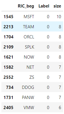
The code below creates the new column to store the first part of the RIC and presents the number of occurrences of each company in our dataset along with its Label.
#add a column to store the first part of the RIC
dataset.insert(loc = 1, column = 'RIC_beg', value = [dataset['instrument'][i].split(".")[0] for i in range(len(dataset))])
dup_df = dataset[['RIC_beg', 'Label']]
# group dataset by the number of duplicates per RIC
dup_df_size = dup_df.groupby(dup_df.columns.tolist(),as_index=False).size().sort_values(by='size', ascending=False)
dup_df_size.head(10)
Below, let's also count the number of duplicates per class and see what percentage of the total class dataset the duplicates represent.
target_count = dataset.loc[dataset['Label'] ==1].shape[0]
peer_count = dataset.loc[dataset['Label'] ==0].shape[0]
unique_dup_target = dup_df_size['RIC_beg'].loc[(dup_df_size['size'] > 1) & (dup_df_size['Label'] == 1)].nunique()
unique_dup_peer = dup_df_size['RIC_beg'].loc[(dup_df_size['size'] > 1) & (dup_df_size['Label'] == 0)].nunique()
remove_count_target = dup_df_size.loc[(dup_df_size['size'] > 1) & (dup_df_size['Label'] == 1)]['size'].sum() - unique_dup_target
remove_count_peer = dup_df_size.loc[(dup_df_size['size'] > 1) & (dup_df_size['Label'] == 0)]['size'].sum() - unique_dup_peer
print(f'Number of duplicate RICs in target list is {remove_count_target}')
print(f'Number of duplicate RICs in peer list is {remove_count_peer}')
print(f'{round(remove_count_target/target_count*100,2)}% of target dataset and {round(remove_count_peer/peer_count*100,2)}% of peer dataset will be removed' )
#run remove duplicate function on newly added column and remove that after the function is executed
dataset = dataset.drop_duplicates(subset = ['RIC_beg'], keep = 'first')
Number of duplicate RICs in target list is 1
Number of duplicate RICs in peer list is 842
1.43% of target dataset and 25.29% of peer dataset will be removed
Dealing with missing values
In the next step of Data Preparation, we need to discuss techniques of dealing with the missing values. The most straightforward approach could be the removal of the datapoints with missing values. However, we need to calculate what size of the dataset we are losing in that case and consider the tradeoff between removing the datapoints versus removing the features with many missing values. If the usage of the feature is critical for our model due to a proven high explanatory power, the only option is going to be the removal of the datapoints with the missing values. An additional technique of working with the missing values is the Data imputation when we fill missing values based on mean or median values calculated on the existing datapoints.
Let's now calculate the NaN values per feature for both classes and based on that understand whether we are dropping the datapoints or the features.
print(dataset.loc[dataset['Label']==1].isna().sum())
print('----------------------------------------')
print(dataset.loc[dataset['Label']==0].isna().sum())
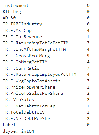
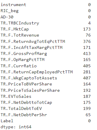
What we can see from the results above the most of NaN carry the current ratio, Working capital to assets, Return on Equity and gross profit margins. As the Gross Profit Margin and the Operating margin are describing the same aspect of the business, we can consider removing Gross Profit Margin. The same considerations work for ROE and ROC allowing us to remove the ROE. As it comes to the current ratio and working capital to assets these are the only variables describing the liquidity aspect of the business. That said we may consider removing one of them but not both.
Below we remove the suggested features to keep many of the datapoints. But before let's also calculate how many datapoints would have been removed if we have conducted a flat drop (without removing features with many NA values).
flat_drop_df = dataset.dropna()
dataset = dataset.drop(columns = ['TR.F.GrossProfMarg', 'TR.F.WkgCaptoTotAssets', 'TR.F.ReturnAvgTotEqPctTTM'])
Then we drop all NaNs from all other features and print dataset shape with flat and the current approach.
print(f'Shape of the dataset after a flat drop - {flat_drop_df.shape}')
dataset = dataset.dropna()
print(f'Shape of the current dataset - {dataset.shape}')
Shape of the dataset after a flat drop - (1688, 20)
Shape of the current dataset - (1801, 17)
As can be seen we have saved 113 datapoints by removing 3 of the features which impact, in fact, is still preserved in our dataset through other proxy features.
Dealing with Outliers
The last thing we look in the guide for the Data preparation phase is the discussing around the outliers. There are multiple techniques on identifying outliers. One of the most used tools in determining outliers is the Z-score which is the number of standard deviations away from the mean that a certain data point is.
The function below calculates the z-score for each datapoint and stores the value in a separate list.
def detect_outlier(df, threshold):
outliers= {}
#calculate mean and standars deviation of the dataset
for column in df:
mean = np.mean(df[column])
std =np.std(df[column])
outliers_list = []
#calculate z-core for each datapoint
for y in df[column]:
z_score = (y - mean)/std
#add the datapoint to outliers list if beyond the threshold
if np.abs(z_score) > threshold:
outliers_list.append(y)
outliers[column] = outliers_list
return outliers
The following function gets the indexes of the outliers which we will further use to remove the outlier datapoints from our dataset.
def getIdx(my_dict):
idxs = {}
for key in outliers.keys():
outlier_idx = []
for item in outliers[key]:
outlier_idx.append(dataset[dataset[key] == item].index.values[0])
idxs[key] = outlier_idx
return idxs
Usually, a datapoint is considered an outlier if it is 3 standard deviations away from the mean, however depending on the use case and the specifics of the dataset different threshold cut-offs can be considered which will obviously result in different number of outliers to be identified and removed.
Below we run the abovementioned function with a threshold ranging from 2 to 3 with 0.2 increment steps.
rng = np.arange(2, 3.1, 0.2)
out_list_total = []
for thresh in rng:
#get outliers and their indexes
outliers = detect_outlier(dataset.iloc[:,4:14], thresh)
outlier_idxs = getIdx(outliers)
#get list of outlier unique indexes to be removed
rem_list = list(outlier_idxs.values())
rem_list = [item for sublist in rem_list for item in sublist]
num_out = len(set(rem_list))
out_list_total.append(num_out)
print(f'Total Number of outliers with threshold {round(thresh,2)}- {num_out}, representing {round(num_out/dataset.shape[0]*100,2)}% of the dataset')
Total Number of outliers with threshold 2.0- 130, representing 7.22% of the dataset
Total Number of outliers with threshold 2.2- 108, representing 6.0% of the dataset
Total Number of outliers with threshold 2.4- 99, representing 5.5% of the dataset
Total Number of outliers with threshold 2.6- 92, representing 5.11% of the dataset
Total Number of outliers with threshold 2.8- 84, representing 4.66% of the dataset
Total Number of outliers with threshold 3.0- 73, representing 4.05% of the dataset
Let's also make a knee plot to see the threshold of the steepest decline in the number of outliers to be removed.
df = pd.DataFrame({'thresh':rng, 'outliers': out_list_total})
fig = px.line(df, y='outliers', x='thresh', markers=True)
fig.show()
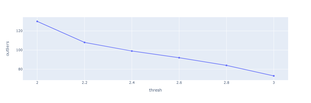
Based on the observation above the steepest decline in the number of outliers is for the threshold 2.2, thus we can use that as a threshold for outlier identification.
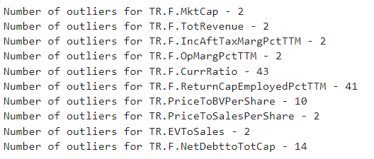
Below we run the function with a threshold of 2.2 and print the number of outliers for each feature
outliers = detect_outlier(dataset.iloc[:,4:14], 2.2)
outlier_idxs = getIdx(outliers)
for key in outlier_idxs.keys():
print(f'Number of outliers for {key} - {len(set(outlier_idxs[key]))}')
Finally, let's drop the outliers with which we conclude the data preparation phase in the scope of this guide.
rem_list = list(outlier_idxs.values())
rem_list = [item for sublist in rem_list for item in sublist]
dataset.drop(set(rem_list), inplace = True)
print(f'The final dataset has the following shape - {dataset.shape}')
The final dataset has the following shape - (1693, 17)
print(f"Number of target companies in trained dataset is: {dataset.loc[dataset['Label']==1].shape[0]}")
print(f"Number of non-target companies in training dataset is: {dataset.loc[dataset['Label']==0].shape[0]}")
Number of target companies in trained dataset is: 55
Number of non-target companies in training dataset is: 1638