ABOUT THE MODEL
The pca_yield_curve.ipynb module performs the PCA decomposition of a user-defined list of rates instruments (e.g. treasuries or IR swaps) and models the expected mean reversion on a given curve trade. Additionally this model runs a Monte Carlo simulation using an Ornstein-Uhlenbeck process to determine the strategy's optimal horizon period, which will be covered later in this article.
This script is designed to be imported as a module into other notebooks using the ipynb python library and used by calling the main calculation function:
| pca_yield_curve.get_data(instruments, strategy, trade) |
The the inputs description is given in the table below:
Parameter |
Description |
Possible arguments |
instruments |
A list of RICs. |
list, e.g. ['US2YT=RR', 'US5YT=RR'] |
strategy |
This parameted should contain the tenors that participate in the trade. |
string, e.g. '5-7-15' or '5-10' |
trade |
The name of the curve trade. There are 2 values supported: 'butterfly' and 'spread' (in case of 2 instruments). |
string |
The function returns a pandas dataframe containing the strategy residual in bps, mean reversion and 2x standard deviation limits; prints out the optimal holding period and builds 2 plotly charts displaying the strategy mean reversion, and the individual residuals by tenors.
DEPENDENCIES AND GLOBAL VARIABLES
Since our model will be consuming Refinitiv data from the Eikon Data API as well as performing linear algebra operations and statistical procedures, we will need to import the following python libraries:
import eikon as ek
import pandas as pd
import numpy as np
import random
import cufflinks as cf
from datetime import datetime, timedelta
from sklearn.decomposition import PCA
from scipy.stats import norm
cf.go_offline()
ek.set_app_key(app_key)
We will not be creating any complex charts, therefore having cufflinks should be sufficient to visualize the reults.
And the following global variables will be used throughout the script:
horizon_date = None
variance_described = 0.0
residuals_values = pd.DataFrame()
residuals_z_scores = []
FUNCTION DEFINITIONS AND MAIN CALCULATION
Apart from the main get_data() function, which will be covered later, the script uses several more custom functions designed to model the mean reversion of the strategy residuals and the estimated optimal holding horizon. These functions are all called after the user initiates the get_data() function - let's have a step-by-step look at the calculation logic.
In this example we will be analyzing a 2s5s10s butterfly curve trade with EU benchmark govies, so our model input will look like this:
instruments = ['EU2YT=RR', 'EU5YT=RR', 'EU10YT=RR']
strategy = '2-5-10'
trade = 'butterfly'
These paramets can then be placed into the get_data() method. Once that is done, the function will initiate with parsing the inputs:
def get_data(instruments, strategy, trade):
global variance_described
global residuals_values
trade_dict = {'spread':1, 'butterfly':2}
if trade_dict[trade] == 2:
pc_limit = 2
else:
pc_limit = 1
_strategy = strategy
strategy = strategy.split('-')
strategy = list(map(lambda x: x+'Y', strategy))
start = datetime.today() - timedelta(days = 365)
. . .
We use a dictionary to classify curve trades by name and choose the respective number of principal components (PCs) that will be used in the subsequent calculations. For a butterfly strategy 2 PCs are used. And we define a start date for the historical timeseries with the help of timedelta to get a 1 year of data. The script then retrieves the timeseries of the selected bonds and calculates the factors (by mean centering of each series) that will be used to calculate the PCs.
tnr, err = ek.get_data(instruments, 'GV4_TEXT')
df = ek.get_timeseries(instruments, 'CLOSE', start_date=start)
df = df.fillna(method='ffill')
df = df.fillna(method='bfill')
df_factors = df.sub(df.mean())
df_diff = df.diff().dropna()
Now that we can use this data with sklearn for eigendecomposition:
pca = PCA(n_components=pc_limit, tol=1e-20, svd_solver='full')
principal_components = pd.DataFrame(pca.fit_transform(df_diff))
eigenvectors = pd.DataFrame(columns=instruments, data = pca.components_)
The above snippet declares that we will be calculating only 2 eigenvectors, and processes the df_diff dataframe (i.e. series of daily changes of the bond yields). Once this is complete, we get a set of eigenvectors:
In [2]:
| eigenvectors |
Out [2]:
| EU2YT=RR | EU5YT=RR | EU10YT=RR | |
| 0 | -0.336137 | -0.571380 | -0.748690 |
| 1 | 0.853164 | 0.151965 | -0.499018 |
And the corresponding eigenvalues are 0.001469 and 0.000162.
NOTE: Mathematically there are several ways of finding the eigenvalues λ and eigenvectors V for a matrix. In this example, we use the series of daily yield changes stored in a pandas dataframe df_diff in order to calculate a covariance matrix C (which is symmetric). This matrix is then factorized using the singular value decomposition approach (SVD). Using sklearn makes this process very easy, and we can validate the results by plugging them into the following equation: VT × C × V = λ, to match the following results: |
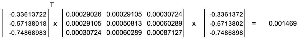
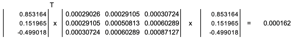
We can also check the orthogonality of these eigenvectors by multiplying each of them pairwise as V1T × V2, which will give us a result of 0.
We will see the variance described by these principal components as we call the pca.explained_variance_ratio_ - in our case thee top 2 components explain 97.72% of the bond yield changes. The matrix multiplication in the snippet below calculates factor loadings by multiplying each row of daily centered yield changes by an eigenvector. This will be used in the calculation of the strategy residuals later.
df_pc = pd.DataFrame()
for i in range(pc_limit):
_pc = []
for j in range(len(df_factors)):
_pc.append(np.dot(eigenvectors.iloc[i,:].values, df_factors.iloc[j,:].values))
df_pc[i] = _pc
df_pc.index = df_factors.index
principal_components = df_pc
principal_components.index = df_factors.index
principal_components = principal_components.T
variance_described = pd.DataFrame(pca.explained_variance_ratio_).sum()
eigenvalues = pd.DataFrame(pca.explained_variance_)
Before we proceed, let’s set the background on the meaning of these residuals, and what role does the choice of PCs play in the calculations.
The purpose of applying PCA to financial markets is to explain the price changes of different assets through a smaller set of factors. This is achieved via the dimensionality reduction of our observations, e.g. instead of looking at 100 factors impacting a price, we can pick just 5, 7, 10 or any other number of “meaningful” factors explaining most of those price changes. For yield curve analysis it is a common practice to use the top 3 principal components, as they describe the following parameters of the yield curve:
- level (PC 1),
- slope (PC 2),
- twist (PC 3).
Isolating these components helps modeling the specific curve movements such as parallel shifts, flattening / steepening as well as changes to its overall curvature. This is the reason why our strategy choice affects the number of used components.
Example: if we are building a curve spread strategy (e.g. flattener), we would like to isolate the shift and focus only on the changes to its slope, whereas if we are dealing with a butterfly trade, we will attempt to isolate both the shift and the slope changes, so that we can capture changes in the curvature.
To achieve this, we calculate the strategy residuals by taking the demeaned (centered) daily yield changes and deducting the pairwise multiplications of the loading factors and the required number of PCs. Since we are modelling a butterfly trade, our formula looks like this:
Residualt[T] = Demeaned_Chgt[T] – Factor1t× PC1[T] – Factor2t× PC2[T],
where t is the timestamp of the historical series, T is the tenor of the bond, while PC1 and PC2 are the respective values of 1st and 2nd eigenvectors corresponding to the bond maturing at T. This is how the above is implemented in the script:
residuals = pd.DataFrame(columns=instruments)
for i, r in df_factors.iterrows():
_v = []
for c in eigenvectors.columns:
_v.append(np.dot(eigenvectors[c], principal_components[i]))
_res = pd.DataFrame(np.subtract(r.values, _v))
_res.index = instruments
_res.columns = [i]
_res = _res.T
residuals = residuals.append(_res)
_tnr = list(map(str.strip, tnr['GV4_TEXT'].values.tolist()))
residuals.columns = _tnr
residuals_values = residuals * 100
We then calculate the butterfly residual similarly to the yield:
ResidualStrategy = Residual1 – 2 × Residual2 + Residual3
if len(strategy) == 3:
df_str = pd.DataFrame(
(residuals[strategy[0]] - (2 * residuals[strategy[1]]) + residuals[strategy[2]])*100)
else:
df_str = pd.DataFrame((residuals[strategy[1]] - residuals[strategy[0]])*100)
MEAN REVERSION
Unlike equity or commodity prices, yields on fixed income products are not expected to grow infinitely – they tend to fluctuate around within some % interval reverting to its mean value over a period of time. The same logic applies to their residuals. But what are the specifics of this mean reversion? How quick will it happen? This python model addresses these questions by calculating:
- the projected mean reversion within a 2 × standard deviation corridor;
- an optimal holding horizon date.
df_mrv = getMeanReversion(df_str)
We will be using the Ornstein-Uhlenbeck model to construct the regression. Our script uses the strategy residuals timeseries as an input for the getMeanReversion() function, which starts with a call to a mean reversion parameter calculation as follows:
def getMeanReversion(_df):
global horizon_date
rv_params = getMeanReversionParams(_df)
Mean = rv_params[0]
Lambda = rv_params[1]
Sigma2 = rv_params[2]
. . .
The getMeanReversionParams() function returns an array of the Ornstein-Uhlenbeck parameters: μ (mean), λ (rate of mean reversion) and σ2 (variance) after fitting them to the input data using the maximum likelihood estimate method. We then calculate the mean reversion trajectory using the formula:
St = St-1 e(-μλ) + μ (1 – e(-λ))
And the two standard deviations boundaries are derived by:
Uppert = St + 2 × SQRT(0.5 σ2 / λ (1 – e(-2 λ t)));
Lowert = St – 2 × SQRT(0.5 σ2 / λ (1 – e(-2 λ t))).
date_array = []
expected = []
upper_2s = []
lower_2s = []
for t in range(252):
_dt = datetime.timestamp(_df.index[-1])
_dt = datetime.fromtimestamp(_dt)
date_array.append(_dt + timedelta(days = t))
if t == 0:
expected.append(_df.iloc[-1][0] * np.exp(-Lambda) + Mean * (1 - np.exp(-Lambda)))
else:
expected.append(expected[t-1] * np.exp(-Lambda) + Mean * (1 - np.exp(-Lambda)))
drift = 0.5 * Sigma2 / Lambda * (1 - np.exp(-2 * Lambda * t))
upper_2s.append(expected[t] + 2 * np.sqrt(drift))
lower_2s.append(expected[t] - 2 * np.sqrt(drift))
The distribution data is stored in a pandas dataframe, which we will plot using cufflinks later. But before the we exit the getMeanReversion() function, we will calculate the optimal holding period for our butterfly strategy by calling the getFPT() method from here:.
holding_horizon = getFPT(_df.iloc[-1][0], Mean, Sigma2, Lambda)
print('Optimal holding period (days): ' + str(round(holding_horizon, 1)))
h_date = datetime.today() + timedelta(days = round(holding_horizon))
print('Horizon date: ' + h_date.strftime('%Y-%m-%d'))
horizon_date = h_date.strftime('%Y-%m-%d')
mrv['Mean Reversion'] = expected
mrv['+2 sigma'] = upper_2s
mrv['-2 sigma'] = lower_2s
mrv.index = date_array
return mrv
The getFPT() function is based on a first passage time approach, which is defined below:
def getFPT(s0, Mean, Sigma, Lambda):
sim = 150
steps = 100
mc = OUMonteCarlo(s0, Mean, Sigma, Lambda, sim, steps)
temp_ftp = countwhile(steps, mc, Mean, sim)
var = 0
if len(temp_ftp) == 0:
var = 0
else:
for i in range(sim):
var += temp_ftp[i][0]
return var / sim
The next snippet defines the Monte Carlo simulation method – OUMonteCarlo() – where we use the stochastic differential equation for the Ornstein-Uhlenbeck process to model the strategy residuals as
dSt = λ (μ - St) dt + σ dWt ,
where Wt is a Wiener process:
def OUMonteCarlo(s0, Mean, Sigma, Lambda, sim, steps):
#simulating an Ornstein-Uhlenbeck process
mc = pd.DataFrame()
for i in range(sim):
_sim = []
for j in range(steps):
if j == 0:
_sim.append(s0)
else:
W = norm.ppf(random.random())
_sim.append(_sim[j-1] * np.exp(-Lambda) + Mean * (1 - np.exp(-Lambda)) + np.sqrt(Sigma) * W) #sqrt dt = 1
mc[i] = _sim
return mc
The returned data would look like this, and we’ll notice that it closely resembles the shape of the derived mean reversion, which will be plotted as we exit the get_data() function:
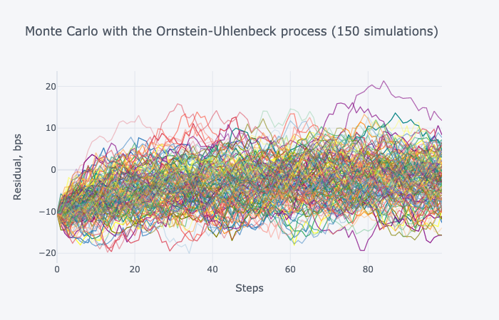
We then go through every simulation and count the number of timesteps until the value of a simulated datapoint exceeds the mean parameter for the first time. The average of these counts is the estimated number of days for the strategy optimal holding horizon.
The above step concludes the analytical part of get_data(), and we exit the function by combining the strategy residual and the mean reversion projections into a single pandas dataframe:
df_str = df_str.rename(columns={0:'Strategy'})
df_mrv['Strategy'] = np.nan
df_str['Mean Reversion'] = np.nan
df_str['+2 sigma'] = np.nan
df_str['-2 sigma'] = np.nan
res_vol = residuals_values.std()
res_mu = residuals_values.mean()
res_last = residuals_values.tail(1)
residuals_z_scores = (res_last - res_mu) / res_vol
df_out = pd.concat([df_str, df_mrv], sort=True)
And the results are displayed with a plotly chart using cufflinks:
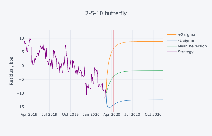
fig1 = df_out.iplot(vline = [horizon_date], yTitle = 'Residual, bps', title = _strategy+' '+trade)
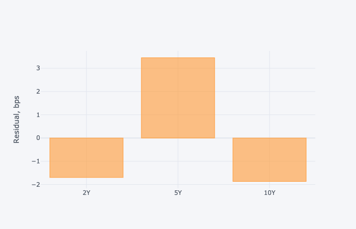
fig2 = residuals_values.tail(1).T.iplot(kind='bar', yTitle = 'Residual, bps')
return df_out
The 2 charts showing the mean reversion with the horizon date, as well as the individual residuals attributed to the bond tenors are presented below.
Out [2]:
| Optimal holding period (days): 26.1 Horizon date: 2020-04-04 |