

According to Investopedia 'Technical Analysis is a trading discipline employed to evaluate investments and identify trading opportunities by analyzing statistical trends gathered from trading activity, such as price movement and volume'. It further states 'technical analysts focus on patterns of price movements, trading signals ... to evaluate a security's strength or weakness'.
According to the various articles etc that I read, three of the more commonly used TA indicators are
- Simple Moving Averages
- Relative Strength Index
- Stochastic Oscillator
Investors and traders who use Technical Analysis as part of their trading strategy may refer to TA charts on a regular basis to help determine their investment choices.
In this workflow, I am going to experiment with how I can use these indicators to generate Buy or Sell trading signals. There are several articles on the internet which attempt the same thing - often focusing on a single indicator - and most of these run the analysis on historical data, present the historical results and stop there.
However, for this workflow I want to take this a step further by continuing to run the analysis on an ongoing basis at a configured interval - e.g. every minute, hour, day (I did look at using realtime tick data as well but it was pointed out that this does not make much sense from a technical analysis perspective - as the ticks do not occur at regular interval).
Furthermore, when a trading signal is generated I will use a chat BOT to post the signal details into a chat room notifying the users - saving the effort of frequently interrogating the charts.
I have access to the Refinitiv Eikon desktop application so I will be using its Data API which can access historical, reference and real-time streaming data. I will also use symbology conversion functions to convert from ISINs to RIC (Reuters Instrument Codes) for requesting the various data. In addition, I will use the Refinitiv Messenger BOT API to post a message to a Refinitiv (Eikon) Messenger Chatroom - no doubt this could easily be replaced with some other form of messaging.
Before we go any further I should mention that I am relatively new to the Eikon Data API and to Python itself - so you may come across some 'not very Pythonic' ways of doing things. If you find some instances which border on sacrilege (in the Python world) please let me know and I will try and amend the offending code.
TA-Lib: Technical Analysis Library
When I started on this, I was using various Python scripts/snippets I found online for calculating my indicators and then wondering just how accurate they may truly be. After spending (wasting?) some considerable time testing and fretting about the veracity of these snippets, a colleague (thank you Jason!) mentioned that there already existed a Python wrapper - ta-lib - for the well known Technical Analysis Library - TA-Lib. Off course - this being Python there would have to be a library for it (remember - Python noob)!
Import our libraries
I think I should mention the versions of some of the key libraries I have installed - just in case you have any issues:
- eikon - 1.1.4
- pandas - 1.1.0
- numpy - 1.19.1
- talib - 0.4.18
- matplotlib - 3.3.1
If you are working on Windows and decide to build the TA-Lib binaries (rather than download the prebuilt ones) pay attention to the instructions on moving the folder (otherwise you may be scratching your head as to why it won't build properly)!
To post messages to the RM Chatroom I am using the existing Messenger BOT API example MessengerChatBot.Python from Github - full details are provided on the site.
Key Code Snippets
As there is a considerable amount of code involved, I will be omitting much of the code here and mostly showing only key code snippets - please refer to the Github repository for the full source code.
So, let me crack on with the code - in the following order:
- various helper functions for the TA, timing and chart plotting
- the main control section
- finishing with the ongoing analysis loop.
Simple Moving Averages
This function uses the TA-Lib SMA function to calculate the Simple Moving Average using the Close price for two periods - which you will note later are 14 for the short period and 200 for the long period. As you will see later, the period interval itself can vary e.g minute, daily, monthly, hourly - so for example, calculate SMA for 14 days and 200 days.
With the calculated SMAs, it then uses the following logic to generate Buy and Sell signals:
- If the short period SMA crosses up through the long period SMA then this is a buy signal
- If the short period SMA crosses down through the long period SMA then this is a sell signal
def SMA(close,sPeriod,lPeriod):
shortSMA = ta.SMA(close,sPeriod)
longSMA = ta.SMA(close,lPeriod)
smaSell = ((shortSMA <= longSMA) & (shortSMA.shift(1) >= longSMA.shift(1)))
smaBuy = ((shortSMA >= longSMA) & (shortSMA.shift(1) <= longSMA.shift(1)))
return smaSell,smaBuy,shortSMA,longSMA
The smaSell and smaBuy Series will contain the date/time and a flag to indicate a signal e.g. for a daily interval you would see something like:
Date
2018-02-15 False
2018-02-16 False
2018-02-19 True
2018-02-20 False
Relative Strength Index
RSI calculation is usually done for a 14 day period - so once again I feed in the Close price for the instrument to the TA-Lib RSI function. The common methodology is to set high and low thresholds of the RSI at 70 and 30. The idea is that if the lower threshold is crossed, the asset is becoming oversold and we should buy. Conversely, if the upper threshold is crossed then the asset is becoming overbought and we should sell.
def RSI(close,timePeriod):
rsi = ta.RSI(close,timePeriod)
rsiSell = (rsi>70) & (rsi.shift(1)<=70)
rsiBuy = (rsi<30) & (rsi.shift(1)>=30)
return rsiSell,rsiBuy, rsi
As per my SMA function, my RSI function also returns a Series containing date/time and a flag to indicate buy/sell signals
Stochastics
The TA-Lib Stoch function returns two lines slowk and slowd which can then be used to generate the buy/sell indicators. A crossover signal occurs when the two lines cross in the overbought region (commonly above 80) or oversold region (commonly below 20). When a slowk line crosses below the slowd line in the overbought region it is considered a sell indicator. Conversely, when an increasing slowk line crosses above the slowd line in the oversold region it is considered a buy indicator.
def Stoch(close,high,low):
slowk, slowd = ta.STOCH(high, low, close)
stochSell = ((slowk < slowd) & (slowk.shift(1) > slowd.shift(1))) & (slowd > 80)
stochBuy = ((slowk > slowd) & (slowk.shift(1) < slowd.shift(1))) & (slowd < 20)
return stochSell,stochBuy, slowk,slowd
We have a Trade Signal - so send it to the Chat Room!
I need a way of letting users know that a Trade signal has been generated by the Technical Analysis. So, I am going to use the Messenger BOT API to send messages to other Refinitiv Messenger users. I am re-purposing the existing MessengerChatBot.Python example from GitHub.
# Key code snippets - see Github for full source
def sendSignaltoChatBot(myRIC, signalTime, indicators):
indicatorList = ','.join(indicators.values)
message = f"TA signal(s) Generated : {indicatorList} at {signalTime} for {myRIC}"
# Connect, login and send message to chatbot
rdp_token = RDPTokenManagement( bot_username, bot_password, app_key)
access_token = cdr.authen_rdp(rdp_token)
if access_token:
# Join associated Chatroom
joined_rooms = cdr.join_chatroom(access_token, chatroom_id)
if joined_rooms:
cdr.post_message_to_chatroom(access_token, joined_rooms, chatroom_id, message)
Run the Technical Analysis
Initially, I will do a historical TA run, after which I will use this function to run the above 3 TA methodologies on the data I get as part of the ongoing live Technical Analysis.
I am going to repeat some of this code later in the main historical TA run loop - purely for ease of reading.
def runAllTA(myRIC, data):
price = data['CLOSE']
high = data['HIGH']
low = data['LOW']
# Simple Moving Average calcs
smaSell,smaBuy,shortSMA,longSMA = SMA(price,shortPeriod,longPeriod)
# Do the RSI calcs
rsiSell,rsiBuy,rsi = RSI(price,shortPeriod)
# and now the stochastics
stochSell,stochBuy,slowk,slowd = Stoch(price, high, low)
# Now collect buy and sell Signal timestamps into a single df
sigTimeStamps = pd.concat([smaSell, smaBuy, stochSell, stochBuy, rsiSell, rsiBuy],axis=1)
sigTimeStamps.columns=['SMA Sell','SMA Buy','Stoch Sell','Stoch Buy','RSI Sell','RSI Buy']
signals = sigTimeStamps.loc[sigTimeStamps['SMA Sell'] | sigTimeStamps['Stoch Sell'] |
sigTimeStamps['RSI Sell'] | sigTimeStamps['SMA Buy'] |
sigTimeStamps['Stoch Buy'] | sigTimeStamps['RSI Buy']]
# Compare final signal Timestamp with latest data TimeStamp
if (data.index[-1]==signals.index[-1]):
final = signals.iloc[-1]
# filter out the signals set to True and send to ChatBot
signal = final.loc[final]
signalTime = signal.name.strftime("%Y-%m-%dT%H:%M:%S")
indicators = signal.loc[signal].index
sendSignaltoChatBot(myRIC, signalTime, indicators)
If the timestamp of the final TA signal, matches the timestamp of the most recent data point - then we have one or more new trade signal(s) - so inform the Chatroom users via the Chat BOT.
Timing Helper functions
I also need a few helper functions to calculate some time values based on the selected interval - the main one is...
# Calculate Start and End time for our historical data request window
def startEnd(interval):
end = datetime.now()
start = {
'minute': lambda end: end - relativedelta(days=5),
'hour': lambda end: end - relativedelta(months=2),
'daily': lambda end: end - relativedelta(years=2),
'weekly': lambda end: end - relativedelta(years=5),
'monthly': lambda end: end - relativedelta(years=10),
}[interval](end)
return start.strftime("%Y-%m-%dT%H:%M:%S"),end.strftime("%Y-%m-%dT%H:%M:%S")
Plotting functions
Whilst not essential to the workflow, I wanted to plot a few charts to provide a visual representation of the various TA indicators - so we can try and visually tie-up instances where a price rises or drops in line with a TA trade signal - so for example when the short SMA crosses up through the long SMA, do we see an upward trend in the price after that point in time?
# As per before, key code snips only...
# Use a formatter to remove weekends from date axis
# to smooth out the line.
class MyFormatter(Formatter):
def __init__(self, dates, fmt='%Y-%m-%d'):
self.dates = dates
self.fmt = fmt
def __call__(self, x, pos=0):
'Return the label for time x at position pos'
ind = int(round(x))
if ind>=len(self.dates) or ind<0: return ''
return self.dates[ind].strftime(self.fmt)
# Plot the Close price and short and long Simple Moving Averages
def plotSMAs(ric,close,sma14,sma200,sell,buy):
x = close.index
plt.rcParams["figure.figsize"] = (28,8)
fig, ax = plt.subplots(facecolor='0.25')
ax.plot(np.arange(len(x)),close, label='Close',color='y')
ax.plot(np.arange(len(x)),sma14,label="SMA 14", color='g')
ax.plot(np.arange(len(x)),sma200,label="SMA 200", color='tab:purple')
plt.show()
# Plot the Close price in the top chart and RSI in the lower chart
def plotRSI(ric,close,rsi):
plt.rcParams["figure.figsize"] = (28,12)
fig = plt.figure(facecolor='0.25')
gs1 = gridspec.GridSpec(2, 1)
# RSI chart
ax = fig.add_subplot(gs1[1])
ax.xaxis.set_major_formatter(formatter)
ax.plot(np.arange(len(rsi.index)), rsi.values,color='b')
plt.axhline(y=70, color='w',linestyle='--')
plt.axhline(y=30, color='w',linestyle='--')
# Close Price chart
axc = fig.add_subplot(gs1[0])
axc.plot(np.arange(len(rsi.index)), close, color='y')
plt.show()
# Plot Close price in top chart and in the slowk + slowd lines in lower chart
def plotStoch(ric,close,slowK,slowD):
plt.rcParams["figure.figsize"] = (28,12)
fig = plt.figure(facecolor='0.25')
gs1 = gridspec.GridSpec(2, 1)
ax = fig.add_subplot(gs1[1])
# Stochastic lines chart
ax.plot(np.arange(len(slowk.index)), slowk.values,label="Slow K",color='m')
ax.plot(np.arange(len(slowk.index)), slowd.values,label="Slow D",color='g')
plt.axhline(y=80, color='w',linestyle='--')
plt.axhline(y=20, color='w',linestyle='--')
# Closing price chart
axc = fig.add_subplot(gs1[0])
axc.plot(np.arange(len(close.index)), close, color='y')
plt.show()
So, that's the helper functions out of the way - let's move on the main control section
Connecting to the Eikon application
To connect to my running instance of Eikon (or Workspace) I need to provide my Application Key.
ek.__version__
ek.set_app_key('<your app key>')
Some initialisation code
I need to calculate the start and end date for my price query - based on the chosen periodicity/interval, as well as specify the periods for moving averages.
Also, as I will be requesting the price of each instrument individually, I create a container to hold all the price data for the full basket of instruments.
Finally, I set some display properties for the Pandas dataframe.
myInterval = 'daily' # 'minute', 'hour', 'daily', 'weekly', 'monthly'
myStart, myEnd = startEnd(myInterval)
timestampLen = timeStampLength(myInterval)
print(f'Interval {myInterval} from {myStart} to {myEnd} : Timestamp Length {timestampLen}')
shortPeriod = 14
longPeriod = 200
basket={}
# Do we want to plot charts?
plotCharts = True
# Dataframe display setting
pd.set_option("display.max_rows", 999)
pd.set_option('precision', 3)
Interval daily from 2018-03-11T11:08:38 to 2020-03-11T11:08:38 : Timestamp Length 10
TA Analysis summary output
Once the initial historical TA has been run, I want to present a summary table of the signal over that period.
For this, I am going to use a Dataframe to output the results in a readable format.
I am also creating some blank columns which I will use for padding the dataframe later.
outputDF = pd.DataFrame(columns=['RIC','Name','ISIN','Close','Periodicity','Intervals Up',
'Intervals Down','Unchanged','1wk %ch','1M %ch','YTD %ch','6M %ch',
'1yr %ch','SMA Sell','SMA Buy','Stoch Sell','Stoch Buy','RSI Sell', 'RSI Buy' ])
blankSignalCols = ['N/A']*6
blankNonSignalCols = [' ']*13
Convert my ISIN symbols to RICs
Whilst Eikon can accept various Symbology types for certain interactions, I need to specify RICs (Reuters Instrument Code) for much of the data I intend to access.
Therefore, I could just start with a bunch of RICs - but not everyone works with RICs - so here is an example of symbology conversion at work.
myISINs = [
'GB0002634946',
'GB00B1YW4409'
]
myRICs = ek.get_symbology(myISINs, from_symbol_type='ISIN', to_symbol_type='RIC')
Just for your reference, the get_symbology function can accept from and to symbol types of
- CUSIP
- ISIN
- SEDOL
- RIC
- ticker
- lipperID
- IMO
In addition, you can also convert to the 'OAPermID' type.
Snapshot some summary data values
Once I have run the TA I want to present a summary table reflecting the price changes for each instrument over various periods such as a week, month, year etc - along with the TA results.
So, for this, I am using the get_data method to obtain various Percent price change values as well the name of the corporate entity and the most recent Closing price
listRICs = list(myRICs.RIC)
pcts, err = ek.get_data(
instruments = listRICs,
fields = [
'TR.CommonName',
'TR.CLOSEPRICE',
'TR.PricePctChgWTD',
'TR.PricePctChgMTD',
'TR.PricePctChgYTD',
'TR.PricePctChg6M',
'TR.PricePctChg1Y',
]
)
pcts.set_index('Instrument',inplace=True)
In the above call, I am requesting each instrument's per cent Price change for Week, Month and Year to Date - and the 6m and 1yr period as well.
Putting it all together for our initial 'historical' analysis run
I can now go ahead and request my historical data and perform the Technical Analysis.
As well as interval data at the minute, hour, daily etc Eikon product can also provide tick data - i.e. individual trades as well as Bid//Ask changes. However, there are some differences in the data set for tick data compared to the other intervals:
- Historical tick data will be indexed on the date+time of every tick - and therefore the index can vary across instruments
- Intervalised data will be indexed according to the interval e.g. every minute, hour etc and therefore use the same index values across multiple instruments
- I can get high, low prices for interval data (which is needed for the Stochastic TA) but not for tick data
As you can see, since the tick data is not interval based, it does not make sense from a TA point of view. For interval data, I can specify multiple RICs in the get_timeseries call and get back a single dataframe with the prices for all the RICs. However, to make the code easier to read, I will loop through the RICs and request each one individually rather than slightly increased subsequent complication involved if I have to use a single dataframe containing all the data.
I have split the following section of code into smaller chunks for ease of reading and annotations.
For each RIC code in our list, the first thing I do is use the get_timeseries function to request a subset of fields at the specified Interval for the previously calculated time period.
for ISIN, symb in myRICs.iterrows():
myRIC=symb['RIC']
data = ek.get_timeseries(myRIC,
fields = ['CLOSE','HIGH','LOW'],
start_date=myStart,
end_date=myEnd,
interval = myInterval)
price = data['CLOSE']
high = data['HIGH']
low = data['LOW']
basket[myRIC]=data # Save each instrument's raw data for later use
Next, I calculate values for Price Up, Down and no change movements for the analysis period. Then I call the various TA functions to calculate the indicators and generate the signals (& plot charts if enabled).
# Count Price Up, Down and No change
upCnt = (price < price.shift(1)).value_counts().loc[True]
downCnt = (price > price.shift(1)).value_counts().loc[True]
try:
ncCnt = (price == price.shift(1)).value_counts().loc[True]
except KeyError as e:
ncCnt = 0
# Do the Simple Moving Average calcs
smaSell,smaBuy,shortSMA,longSMA = SMA(price,shortPeriod,longPeriod)
if plotCharts:
plotSMAs(myRIC,price,shortSMA,longSMA,smaSell,smaBuy)
# Do the RSI calcs
rsiSell,rsiBuy,rsi = RSI(price,shortPeriod)
if plotCharts:
plotRSI(myRIC,price,rsi)
# Stochastic calcs
stochSell,stochBuy,slowk,slowd = Stoch(price, high, low)
if plotCharts:
plotStoch(myRIC,price,slowk,slowd)
# Get the Percent Change data for thisRIC
pct = pcts.loc[myRIC]
Finally, I use the data and signals etc to generate a dataframe displaying a Summary Table of the various stats + any signals generated for our configured TA time period and interval.
# Now we build the summary table
# starting with the non-trade signal related stuff
nonSignalData = [myRIC,
pct['Company Common Name'],
ISIN,
pct['Close Price'],
myInterval,
upCnt,downCnt,ncCnt,
pct['WTD Price PCT Change'],
pct['MTD Price PCT Change'],
pct['YTD Price PCT Change'],
pct['6-month Price PCT Change'],
pct['1-year Price PCT Change']]
# Now build the Signal buy and sell columns for each TA indicator
sigTimeStamps = pd.concat([smaSell, smaBuy, stochSell, stochBuy, rsiSell, rsiBuy],axis=1)
sigTimeStamps.columns=['SMA Sell','SMA Buy','Stoch Sell','Stoch Buy','RSI Sell','RSI Buy']
signals = sigTimeStamps.loc[sigTimeStamps['SMA Sell'] | sigTimeStamps['Stoch Sell'] |
sigTimeStamps['RSI Sell'] | sigTimeStamps['SMA Buy'] |
sigTimeStamps['Stoch Buy'] | sigTimeStamps['RSI Buy']]
# If any trade signals were generated for our time period
# add them to the summary table
signalCnt = len(signals)
if (signalCnt):
first = True
for index,row in signals.iterrows():
sigDate = str(index)[0:timestampLen]
signalList = [sigDate if item else "" for item in row]
# First row to contain non-signal stuff, subsequent rows only trade signals
tempRow = nonSignalData.copy() if first else blankNonSignalCols.copy()
tempRow.extend(signalList)
s = pd.Series(tempRow, index=outputDF.columns)
outputDF = outputDF.append(s,ignore_index=True)
first=False
else: # No signals so just the non-signal related stuff
tempRow = nonSignalData.copy()
tempRow.extend(blankSignalCols)
outputDF = outputDF.append(tempRow)
outputDF.head(5)
outputDF.tail(5)
Once that is done, I simply display the head and tail of the Summary Table.
Before we get to the table, let us have a quick look at the charts I plotted and compare them to the subset of TA signals in the table displayed further down.
Here I have included
- the SMA, RSI and Stochastic charts for the final RIC - III.L
- the head of the outputDF dataframe - showing the first few trading signals for BAE Systems (BAES.L)
- the tail of the outputDF dataframe which represents the final few signals for 3I Group (III.L).
Simple Moving Average chart for 3I Group PLC - III.L
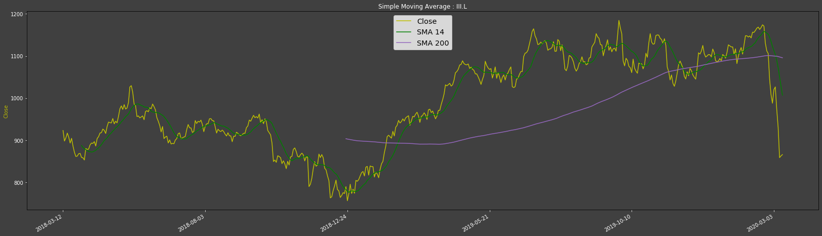
Towards the end of the Simple Moving Average chart, you can see that the SMA14 crosses down through the SMA200 line which is a sell indicator - and if you refer to the tail end of the Summary table below you will see an SMA Sell indicator for the 5th of March 2020.
Relative Strength Index chart for 3I Group PLC - III.L
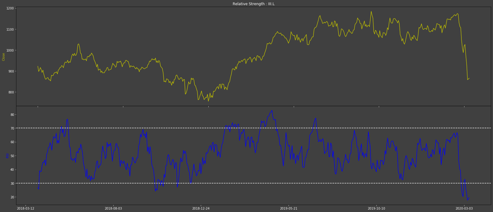
Here I am plotting the Close price in the upper chart and the RSI value in the lower chart. Just at the tail end, you can see that the RSI value crosses below the lower threshold twice around the end of Feb / start of March - which corresponds to the RSI Buy indicators on 2020-02-27 and 2020-03-05 in the Summary table below
Stochastics chart for 3I Group PLC - III.L
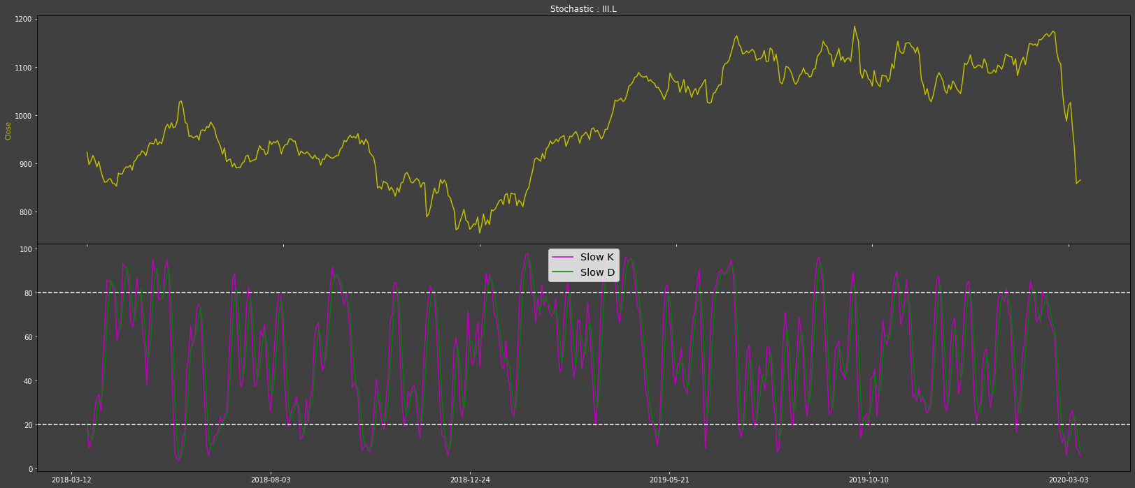
Once again I am plotting the Close price on top and the Stochastics slowk and slowd lines in the lower chart. You can see that the slowk line crosses above the slowd line in the oversold region (below 20) on two occasions - i.e. buy indicators reflected in the summary table below with Stochastic Buy entries for 2020-02-28 and 2020-03-03.
Historical Summary table
After the initial Technical Analysis run using the historical data, I output a historical Summary table with some basic stats as well as the history of the Trade signals for the configured Interval and Time Period.
For the basic stats, I display the Percent change for various periods such as Week to Day, Month to Day, 6 months - to provide an indication of just how the particular stock has been trading over those periods. I also display the number of intervals where the price has gone up, down or no change as potentially useful reference points.
The rightmost columns of the table contain the Buy and Sell signals occurrences for the 3 TA methodologies - one row for each date/time that triggered a signal - you may occasionally see more than one signal in a single row. For example, whilst I was testing both RSI and Stoch indicated Buy signals on 11th October 2018 for the 3i Group (III.L) - concerning this, you may find the Reuters 3 yr chart for III interesting...
Head of the Summary table - showing the first few trading signals for BAE Systems (BAES.L)
RIC |
Name |
ISIN |
Close |
Periodicity |
Intervals Up |
Intervals Down |
Unchanged |
1wk %ch |
1M %ch |
YTD %ch |
6M %ch |
1yr %ch |
SMA Sell |
SMA Buy |
Stoch Sell |
Stoch Buy |
RSI Sell |
RSI Buy |
BAES.L |
BAE Systems PLC |
GB0002634946 |
551 |
daily |
231 |
268 |
7 |
-7.77 |
-9.47 |
-2.48 |
-3.03 |
18.5 |
2018-03-27 |
|||||
2018-04-11 |
||||||||||||||||||
2018-05-11 |
||||||||||||||||||
2018-05-15 |
||||||||||||||||||
2018-05-16 |
The tail of the Summary table - showing the most recent trading signals for 3I Group (III.L)
RIC |
Name |
ISIN |
Close |
Periodicity |
Intervals Up |
Intervals Down |
Unchanged |
1wk %ch |
1M %ch |
YTD %ch |
6M %ch |
1yr %ch |
SMA Sell |
SMA Buy |
Stoch Sell |
Stoch Buy |
RSI Sell |
RSI Buy |
III.L |
3i Group PLC |
GB00B1YW4409 |
863 |
daily |
237 |
262 |
7 |
-7.29 |
-14.4 |
-21.4 |
-23.5 |
-8.45 |
2018-03-27 |
|||||
2020-02-27 |
||||||||||||||||||
2020-02-28 |
||||||||||||||||||
2020-03-03 |
||||||||||||||||||
2020-03-05 |
2020-03-05 |
Note how the final few signals compare with the crossover points on the corresponding charts.
Ongoing Technical Analysis
Now that I have the historical analysis out of the way, I will move onto the ongoing live analysis. In other words, the code that I can keep running to perform the TA on an ongoing basis at the configured interval.
while True:
gotoSleep(myInterval)
for myRIC in listRICs:
historical = basket[myRIC]
latest = ek.get_timeseries(myRIC,fields = ['CLOSE','HIGH','LOW'],
count = 1, interval = myInterval)
# Delete earliest data point
historical.drop(historical.index[0])
# Append latest data point
historical = historical.append(latest)
runAllTA(myRIC, historical)
# Udpate basket with latest values
basket[myRIC] = historical
I put the script to sleep for our configured interval, and when it wakes I request the latest data points for each RIC.
The simplest approach would be to just make the above get_timeseries calls with a revised start_date and end_date parameters. However, this would be quite wasteful of resources and so I will request just the latest data point for my configured interval.
To do this, I make the call with count=1 (rather than Start/End times) to get just the latest data point. I then drop the earliest data point from our historical data points and append the latest one.
I can then invoke the Technical Analysis with the most recent data included.
Closing Summary
I could now leave this script running with my preferred interval and it will send messages to the chatroom, each time the Technical Analysis yields a Buy or Sell signal, like the ones shown below:
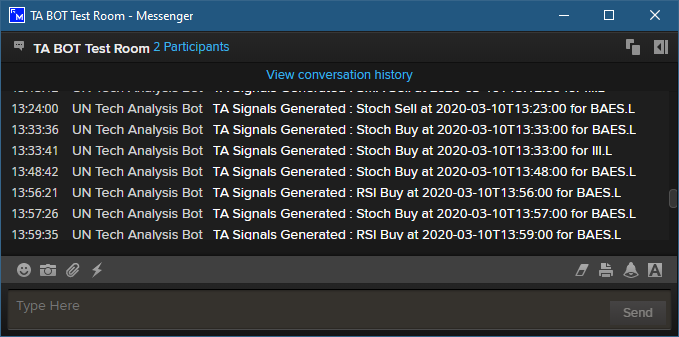
Note: For the purpose of the above screen capture, I did a run with the interval set to 'minute' - in an attempt to generate signals sooner rather than later.
For a trader who uses Simple Moving Average, Relative Strength Indices and/or Stochastic charts to help inform their trading decisions - this could mean they don't need to actively sit there eyeballing charts all day long.
I hope you found this exercise useful and no doubt there are many possible improvements/refinements that could be made to both the code and the simple TA methodology I have used. A few examples to consider are:
- In the Summary table extract above I can see that on 2020-03-05, SMA based TA is indicating a Sell whereas the RSI based TA is indicating a Buy - which suggests that further refinements are required
- An RSI related article I read, suggested that once the line crosses a threshold it may be better to wait till it crosses back in the opposite direction before generating a signal - so for example, if the crosses below %30, wait till it crosses back up above 30% before generating a Buy signal.
- In my summary output table, I show the '% change' for a week, month, year etc - which could be relevant for my 'daily' interval-based TA - but not so much if say I used an 'hourly' interval. My colleague (Jason again) suggested that a better approach could be to show '% change' values for say, Hour t, Hour t+1, t+5, t+10 etc according to my chosen interval.
- Another improvement could be to show up/down markers on the plot lines highlighting the crossover points.
As you can expect, there is no shortage of material on Technical Analysis to be found on the internet.
NOTE: I do not endorse the above workflow as something that should be used for active trading - it is purely an educational example.
References
You will find links to Source Code, APIs and other related articles in the Links Panel.